The entropy of a discrete variable can be defined as
$$H(x) = - \sum_{i=1}^n p(x) \log p(x) $$
or for continuous distributions and a density $f(x)$ we could compute
$$h[f] = \int_{\mathbb{X}} f(x) \log f(x) \, dx$$
In the case of an observation of a sample from a distribution of a discrete variable, we could compute an observed entropy. This is for instance the basis behind a G-test.
Question: Is there a similar expression of entropy for an observed set of points, when the variable is continuous?
Motivation: Based on this question Kolmogorov Smirnov Test : CDF vs PDF I wondered whether there could be a test that does not depend on comparing the empirical distribution function with the CDF but instead on some comparison of the spread of points.
Say we have a sample that is distributed according to a uniform distribution (the distribution of quantiles for any continuous distribution). Then intuitively I find a sample from the uniform distribution more 'uniform' than a sample from, say, a Beta(2,2) distribution (which is more concentrated in the center).
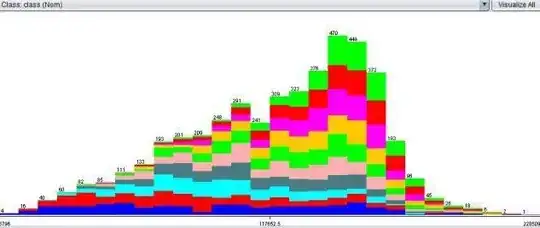
I tried creating some sort of empirical density function from which an entropy could be computed by taking the midpoints between the data points and defining the density in between those midpoints as $1/d$ where $d$ is the distance between the midpoints. For instance, this looks like this:
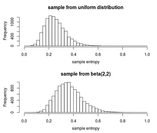
This seems to be no bad approach. When I compare the entropy of this empirical density for ten thousand samples (each of size 30) from a uniform distribution and ten thousand samples from a beta(2,2) distribution, then a 95% hypothesis test has a power around 30% to detect that the sample is not from a uniform distribution. The Kolmogorov Smirnov test has only 10% power.
Has this approach been described and refined in literature?
example code
mids = function(x) {
  l = length(x)
  xo = x[order(x)]                      ### order sample
  xm = (tail(xo,l-1)+head(xo,l-1))/2    ### midpoints
  xm = c(0.5*(head(xo,1)+tail(xo,1)-1), ### add extra points at beginning and tail (wrapping)
         xm,
         0.5*(head(xo,1)+1+tail(xo,1)))
  return(xm)
}

entropy = function(x) {
  l = length(x)

  xms = mids(x)      ### midpoints
  xd = diff(xms)     ### compute distances
  xf = (1/xd/l)      ### compute empirical density

  entropy = sum(xd*xf*log(xf))   ### entropy based on empirical density

  return(entropy)
}

set.seed(1)
n = 30
b1 = 2
b2 = 2
nt = 10^4
### compute entropy from samples
s1 = replicate(nt,entropy(runif(n)))
s2 = replicate(nt,entropy(rbeta(n,b1,b2)))

### plot results
layout(matrix(1:2,2))
par(mar = c(4,4,3,1))
hist(s1, breaks = seq(0,1,0.025), xlab = "sample entropy",
     main = "sample from uniform distribution")
hist(s2, breaks = seq(0,1,0.025), xlab = "sample entropy",
     main = "sample from beta(2,2)")

### power of 95% hypothesis test
sum(s2 >= quantile(s1,0.95))/nt

### power of 95% hypothesis test with Kolmogorov Smirnof test
pks = replicate(nt,ks.test(rbeta(n,b1,b2),punif))
sum(pks<0.05, na.rm = 1)/nt


