We know there are two estimators for the variance of the normal distribution, $s^2$ which is unbiased and $\hat{\sigma}^2$ which is biased, but does better on the mean squared error criterion (see here). Is it better for this contest to use $\hat{\sigma}^2$ due to this?
No,
Or at least, optimizing squared error (or absolute error since it is about the smallest absolute error who wins), is not a uniform best winning strategy (it does not win from all other strategies).
Bias with shrinking and biased estimators with lower mean error
Say, we use only the standard error computed as
$$s^2 = \frac{1}{n-1} \sum{(x_i-\bar{x})^2}$$
It is the sufficient statistic and other data are not more helpful. (in the simulations below we simulate this by drawing from a chi-squared distribution)
We can use estimators with a particular scaling.
$$\hat\sigma^2_f = f s^2$$
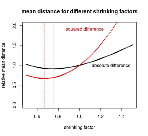
If $f=1$ then we have the unbiased estimator. But as we see in the figure below, it is a lower value of $f$ that performs better (has a lower error in terms of mean squared error or mean absolute error).
The figure below is computed for sample size $n = 5$.
See also here for a demonstration of this shrinking factor: Bias / variance tradeoff math
Lowest mean error is not necessarily the best strategy
It is not about making the smallest possible mean error.
Instead, it is about making often a smaller error (that's what makes you win from opponents). It is better to have very small errors combined with very large errors, than only medium errors. Even when the latter is on average better.
Below we see the performance of alternative strategies, in the situation that all your opponents use the strategy that aims for the lowest mean error.
If we use the same strategy as the opponents (the vertical lines), then we all have the same strategy and have all equal chances to win (the figure is for 3 opponents, 4 contestants in total so 25% win percentage).
We see that using less shrinking, will improve the win percentage. With less shrinking the mean error is bigger, but this is countered by being more often very close (we do not care if for some percentage we make extremely large errors, optimizing those is not gonna make us win).
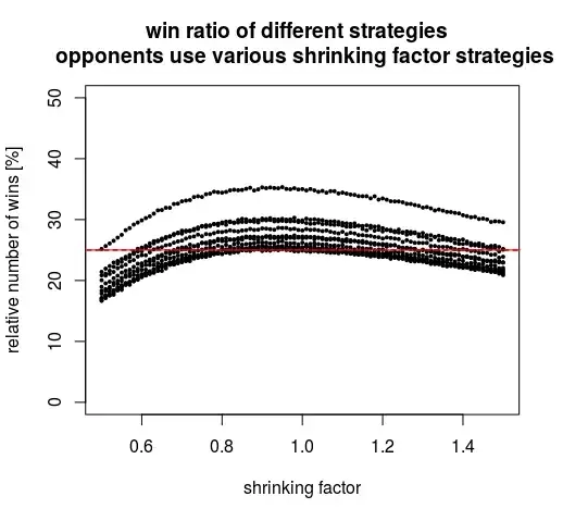
The above graph is the situation when your three opponents use the lowest mean distance strategy (either based on lowest mean square distance or lowest mean absolute distance). But what if they would do something else? The graph below plots the situation but now instead of two curves we plot eleven curves where for each curve the opponents use a different shrinking factor (from 0.5 to 1.5 in steps from 0.1, giving 11 curves). You see that a shrinking factor a bit above 0.9 is giving the best result, no matter what the opponents do. In the worst case, the opponents choose the same strategy and you all have an equal probability to win.
Wrap up
The above is simulations. They show at least that minimizing the mean squared error is not necessarily the best strategy.
But, in order to compute which strategy is best, you would need to perform more simulations. Ideally one would be able to write formulas (it would be something with order distributions) such that no computations are necessary.
If there is an optimal strategy then it probably aims to optimize a small percentage of the guesses (a fraction a bit above 1/n where n is the number of opponents) to be with a very small distance. We do not care if in the rest we make huge errors.
With some testing for other numbers of opponents, it seems that the more opponents you have, the more the optimal strategy shifts towards the unbiased estimate with $f=1$.
- With few opponents it is better to optimize the mean error and use a biased estimate.
- With many opponents it is better to minimize the bias (which increases the frequency of small errors, at the cost of some very large errors).
computer code for simulations and graphs
### init
set.seed(1)               # set random seed for reproducibility
m = 10^5                  # number of samples to compute statistics
nu = 4
x = rchisq(m,nu)          # draw sample from chi-squared distribution
                          # this is the sum of squares that you get
                          # from nu+1 normal distributed samples

fs = seq(0.5,1.5,0.01)    # parameter of shrinking factors that we are gonna test

sy = sum(abs(x-4))        # compute absolute deviation error of non biased estimator
sy2 = sum(abs(x-4)^2)     # compure squared error of non biased estimator


### function to compute absolute deviation error
### of biased estimator (shrinking with a factor fi)
reld = function(fi) {
  sum(abs(fi*x-4))/sy
}
reld = Vectorize(reld)

### function to compute squared deviation error
### of biased estimator (shrinking with a factor fi)
reld2 = function(fi) {
  sum(abs(fi*x-4)^2)/sy2
}
reld2 = Vectorize(reld2)

### plot error comparison of biased estimators with unbiased estimator
plot(-10,-10, xlim = c(0.5,1.5), ylim = c(0,2),
     ylab = "relative mean distance", xlab = "shrinking factor",
     main = "mean distance for different shrinking factors")
y1 = reld(fs)
y2 = reld2(fs)
points(fs, y1, pch = 21, col = 1, bg = 1, cex = 0.4)
points(fs, y2, pch = 21, col = 2, bg = 2, cex = 0.4)

text(1.3,1, "absolute difference")
text(1.05,1.9, "squared difference", col =2)


### lines of the optimum
x1 = fs[which.min(y1)]
lines(x1*c(1,1), c(-1,3), lty = 2)
x2 = fs[which.min(y2)]
lines(x2*c(1,1), c(-1,3), col = 2, lty = 2)

### function to get the best result (distance) from n oponents
sim = function(fi,n) {
  x = matrix(rchisq(m*n,nu),m)       ### measurements of your opponents
  d = abs(fi*x-nu)                      ### score of opponents if they would use bias fi
  y = apply(d, 1, function(x) min(x))  ### the score of your best opponent
  y
}

### function to get the best result (distance) from n oponents
### same as above but for squared distance
sim2 = function(fi,n) {
  x = matrix(rchisq(m*n,nu),m)
  d = abs(fi*x-nu)^2
  y = apply(d, 1, function(x) min(x))
  y
}

opp = 3
score1 = sim(x1,opp)
score2 = sim2(x2,opp)

### function to test strategy against ensemble
getwins = function(fi) {
  y = sim(fi,1)
  wins = sum(y<score1)  ### count wins
  wins/m           ### compute proportion
}
getwins = Vectorize(getwins)

### function to test strategy against ensemble
getwins2 = function(fi) {
  y = sim2(fi,1)
  wins = sum(y<score2)  ### count wins
  wins/m           ### compute proportion
}
getwins2 = Vectorize(getwins2)


### plot win comparison of different strategies
wins = getwins(fs)
wins2 = getwins2(fs)

plot(-10,-10, xlim = c(0.5,1.5), ylim = c(0,2)*100/(opp+1),
     ylab = "relative number of wins [%]", xlab = "shrinking factor",
     main = "win ratio of different strategies  \n opponents use lowest mean distance strategy")

points(fs,100*wins, pch = 21, col = 1, bg = 1, cex = 0.4)
points(fs,100*wins2, pch = 21, col = 2, bg = 2, cex = 0.4)

lines(c(0,2),c(1,1)*100/(opp+1), lty = 2)
lines(x1*c(1,1), c(-100,300))
lines(x2*c(1,1), c(-100,300), col = 2)

text(1.3,20, "absolute difference")
text(1.2,30, "squared difference", col =2)


