Delta method for estimating a ratio involving variance and mean

Question

Let $X$ be a binomial RV with parameters $(n,p)$. I am interested in the ratio given by $\hspace{5cm}\boxed{R=\frac{var[f(X)]}{\mu[f(X)](1-\mu[f(X)])}}$

where $\mu[f(X)]$ denotes the mean of $f(X)$.

In my case, $f(X)$ is $e^{-\left(\frac{a}{bX+c}\right)}$. The constants $a,b,c$ can take values such that $0 \lt a,b,c \leq 10$.

My aim is to find the value of $p$ that maximize $R$ in terms of $a,b,c$ and $n$. Can someone suggest a simplification to $R$ so that the optimal value for the parameter $p$ can be computed analytically?

My attempt: I was unable to exactly compute the mean and variance of $f(X)$ due to the non-linear form of $f(X)=e^{-\left(\frac{a}{bX+c}\right)}$ . It is not trivial how to take derivatives of $\mu[f(X)]$ and $var[f(X)] $ to optimize for $R$ with this non-linear $f(X)$.. Hence, I thought of using an approximation based on the Taylor series which is known as the delta method) See this and this for reference.)

The approximation to mean $\mathrm{E}[f(X)] \approx f\left(\mu_{X}\right)+\frac{f^{\prime \prime}\left(\mu_{X}\right)}{2} \sigma_{X}^{2}$ worked well when I tried numerically.

However, the approximation for variance given by $Var[f(X)] \approx f^{\prime}(\mu)^{2} \cdot \sigma^{2}+\frac{f^{\prime \prime}(\mu)^{2}}{2} \cdot \sigma^{4}$ seems to be very off from the original values in my numerical simulations. As suggested by jbowman, the variance approximation I am using seems to be of centered-Gaussian. The better approximation seems to me very complicated since I finally want to optimize $p$ to maximize $R$.

It would be great if indeed someone can come up with an expression for the optimal $p$ in terms of $a,b,c,n$ approximately.

Other than the general case, I am also interested in the following scenarios:

small values of $n$, large values of $n$
$\frac{b}{c}>>1$
$\frac{b}{c}<<1$

Please feel free to write an answer even if you can only solve these special cases.

With $n=4$, you only have five outcomes; you can just write the mean and variance of $f(X)$ out explicitly, then $R$, then solve, or so it seems to me. Just out of curiosity, why is $n$ something you can choose? I'd expect the optimal $p$ to be a function of $n$, as the mean and variance of $X$ are. — jbowman, Oct 23 '21 at 22:41
@jbowman , I just considered lower value of $n$ in my simulation. $n$ can be high as well but it is a constant. For example, say n=100 is possible. I am interested in the best $p$ as a function of $a,b,c, n$. I will add this as a note. — wanderer, Oct 23 '21 at 22:44
Also note that your expression for $Var[f(X)]$ is the one for a centered Gaussian distribution, not the general form, which is given in the first answer to your second link. So yes, it will be a poor approximation for small $n$. For larger $n$, if the optimum $p$ is such that the Binomial distribution isn't far from symmetric, it'll be better. — jbowman, Oct 23 '21 at 22:48
This would be easier to read with $Y=f(X)$, and with the standard $E$ (expectation) instead of $\mu$. Then $$R=\frac{var[Y]}{E[Y](1-E[Y]}=\frac{E[Y^2]-E[Y]^2}{E[Y]-E[Y]^2}$$ — Matt F., Oct 26 '21 at 01:06
why do you need/want to use approximations for the expectation and variance? — bdeonovic, Oct 26 '21 at 01:37
@bdeonovic To me, it seemed that it is hard to compute the variance and mean exactly, because of the non-linearity of $f(X)=e^{-\frac{a}{bX+c}}$. — wanderer, Oct 26 '21 at 02:01
As an example, for $n=10, a=2, b=1, c=2$, the maximum $R$ comes from $p=0.15$. — Matt F., Oct 26 '21 at 02:11
the mean and variance is relatively easy to compute, eg. $Ef(X) = \sum_x f(x)*P(X=x)$ where $P(X=x)$ is the binomial pmf and the sum is over $0,\ldots,n$. The hard part is taking derivatives of $Ef(X)$ and $Varf(X)$ so that you can optimize $R$ — bdeonovic, Oct 26 '21 at 12:22
@bdeonovic ,Yes, that's actually what I meant to convey. I will add that in the question for clarity. — wanderer, Oct 26 '21 at 14:31
@bdeonovic, taking derivatives is easy too. But look at $n=2$: the optimal $p$ is a root of the 5th-degree polynomial $$2 q (p u-p v+q t-q u) \left(2 p^2 v+4 p q u+2 q^2 t-1\right) \\ \left(2 p^2 v (2 p u+q t)+4 p^2 q u^2-p^2 (p+1) v^2+4 p q^2 t u-2 p u^2+q^3 t^2-q t^2\right)-\left(p^2 v+2 p q u+q^2 t-1\right) \left(p^2 v+2 p q u+q^2 t\right)\\ \left(4 (p u-p v+q t-q u) \left(p^2 v+2 p q u+q^2 t\right)-2 p u^2+2 p v^2-2 q t^2+2 q u^2\right)$$ where $q=1-p, t=e^{-a/c}, u=e^{-a/(b+c)}, v=e^{-a/(2b+c)}$, which is a mess. — Matt F., Oct 26 '21 at 17:03
hoping to get an analytical solution is ...wishful thinking. Just use numerical optimization like Newton-Raphson to optimize $R$. No need for approximations — bdeonovic, Oct 26 '21 at 17:09

G. Grothendieck · Accepted Answer · 2021-10-28T14:06:47.417

Calculate the mean and standard error using the delta method via the car R package deltaMethod function which will produce an object with Estimate and SE components, form the required objective function obj and then optimize it as shown in the R code below.

library(car)

obj <- function(p, a, b, c, n) {
  with(deltaMethod(c(x = n*p), "exp(-a / (b*x + c))", n*p*(1-p)),
      SE^2 / (Estimate * (1-Estimate)))
}

# use sample inputs a = b = c = 1; n = 10
out <- optimize(obj, 0:1, maximum = TRUE, a = 1, b = 1, c = 1, n = 10); out
## $maximum
## [1] 0.05530323
##
## $objective
## [1] 0.09935807

curve(Vectorize(obj)(p, a = 1, b = 1, c = 1, n = 10), 0, 1, xname = "p")
with(out, abline(v = maximum, h = objective, lty = 2))

Added

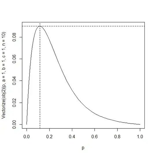
Another approach, not using the delta method, suggested in the comments under the question is to calculate the moments explicitly which we do below. For each of X = 0, 1, ..., n we multiply f(X) by probability of X = x and sum to give the expected value of f(X) and do the same for f(X)^2. Then we form R and optimize the resulting objective function.

obj2 <- function(p, a, b, c, n) {
   f <- function(x) exp(-a / (b*x + c))
   d <- dbinom(0:n, n, p)
   EfX <- sum(f(0:n) * d)
   EfX2 <- sum(f(0:n)^2 * d)
   R <- (EfX2 - (EfX)^2) / (EfX * (1 - EfX))
   R
}
out2 <- optimize(obj2, 0:1, a = 1, b = 1, c = 1, n = 10, maximum = TRUE); out2
## $maximum
## [1] 0.1152665
##
## $objective
## [1] 0.09023062

curve(Vectorize(obj2)(p, a = 1, b = 1, c = 1, n = 10), 0, 1, xname = "p")
with(out2, abline(v = maximum, h = objective, lty = 2))

Added 2

To optimize over p and a for each value of b in 1, 2, ..., 10 define obj2pa which is the same as obj2 except p and a are passed as a single vector pa. Define the control parameter to specify maximization and iterate the appropriate call to optim over the b values. We have used c(p = 0.1, a = 1) as the starting values.

obj2pa <- function(pa, b, c, n) obj2(p = pa[1], a = pa[2], b = b, c = c, n = n)
control <- list(fnscale = -1) # maximize
res <- sapply(c(b = 1:10), function(b) {
  optim(c(p = 0.1, a = 1), obj2pa, b = b, c = 1, n = 10, control = control) |>
   unlist()
})
res

plot(res["value", ] ~ seq(10), type = "o", xlab = "b", ylab = "R")

giving:

                         b1          b2         b3          b4          b5
par.p            0.09978805  0.06862237  0.0572228  0.05084889  0.04660507
par.a            2.39337549  2.54037637  2.7382708  2.92510730  3.09295976
value            0.11979352  0.22136467  0.3022906  0.36735400  0.42059772
counts.function 61.00000000 77.00000000 59.0000000 71.00000000 69.00000000
counts.gradient          NA          NA         NA          NA          NA
convergence      0.00000000  0.00000000  0.0000000  0.00000000  0.00000000
                         b6          b7          b8          b9         b10
par.p            0.04349253  0.04109848  0.03917312  0.03757072  0.03622872
par.a            3.24316833  3.37803880  3.50018805  3.61183913  3.71459240
value            0.46494752  0.50247638  0.53466985  0.56261323  0.58711559
counts.function 69.00000000 75.00000000 75.00000000 67.00000000 67.00000000
counts.gradient          NA          NA          NA          NA          NA
convergence      0.00000000  0.00000000  0.00000000  0.00000000  0.00000000

Thanks for the R code. I'm not too familiar with R software Could you please show me how to modify the code if I need to jointly optimize $a$ and $p$ so as to maximize $R$. And I would be interested in plotting this maximum $R$ value for $c=1, n =10, b=1:1:10$. — wanderer, Oct 28 '21 at 07:33
From the first two plots, it seems that delta method fails to produce a good enough approximation. Specifically, the optimal $p$ is $0.1152665$ whereas the delta method gives us a value of $p=0.055$ . This is around half of $0.1152665$. I am assuming this "halving behavior" is just a coincidence and not a general trend. Do you agree? — wanderer, Oct 28 '21 at 15:27
Yes, it seems that the delta method does not work too well. It might be recoverable if more terms in the Taylor series approximation were used but that would get more complicated to implement since we couldn't rely on the car deltaMethod function. — G. Grothendieck, Oct 28 '21 at 15:32
Yes. I don't want to pursue the extension to the delta method as adding more terms is complicated. And analytically obtaining an optimal $p$ expression is harder as we add more terms. — wanderer, Oct 28 '21 at 15:34
Do you know why there is a slight difference in $par.p$ and $value$ for the $b1$ case in comparison to the results in figure 2 which also corresponds to $b=1$.? — wanderer, Oct 28 '21 at 15:39

Delta method for estimating a ratio involving variance and mean

1 Answers1

Added

Added 2