Confidence interval of the mean of derived random variables

Question

I have two random variables modeled by a Binomial each:

$$X_1 \sim Bin(n_1, p_1)$$

$$Y_1 \sim Bin(n_2, p_2)$$

For each of those random variables I have one observation each. Based on that observation I can estimate $\hat{p_1}$ or $\hat{p_2}$ and calculate a confidence interval for each.

Now, my problem is that I am interested in a quantity derived from $X_1$ and $Y_1$:

$$Z_1 = \log_2 (X_1 / Y_1)$$

So I would like to find an estimation for the mean, and associated confidence interval, of $Z_1$.

I thought that perhaps I could use the found $\hat{p_1}$ and $\hat{p_2}$. I could generate many (e.g., ~$10,000$) random Binomial variates by using $p=\hat{p_1}$ and $p=\hat{p_2}$, respectively.

Then use the computed $10,000$ random variates for $X_1$ and $Y_1$, and apply the definition of $Z_1$ to estimate an empirical distribution for $Z_1$.

Once I have the $10,000$ variates of $Z_1$, can I calculate the so-called large sample confidence interval (see Section 4 of MIT18_05S14_Reading23b.pdf) to derive an estimate for the $E(Z_1)$?

In summary:

1. From one observation $x_1$ and $y_1$, estimate $p_1$ and $p_2$, respectively.
2. Sample many variates from $X_1 \sim Bin(n_1, \hat{p}_1)$ and $Y_1 \sim Bin(n_2, \hat{p}_2)$.
3. Compute the $Z_1$ variates following its definition and the generated variates for $X_1$ and $Y_1$.
4. Finally, calculate the large sample confidence interval of the mean for $Z_1$.

Does this make sense?

EDIT: I see now that this other question is very similar to mine: Numerical estimation of binomial confidence interval.

EDIT2: Could we go with estimating the credible interval for $p$, and then plug that in the Binomial? That's the Beta-Binomial, right? Then I could generate random variates from the Beta-Binomial to find the empirical distribution of $Z_1$ and move on to the calculation of a confidence interval.

library(ggplot2)
library(extraDistr)

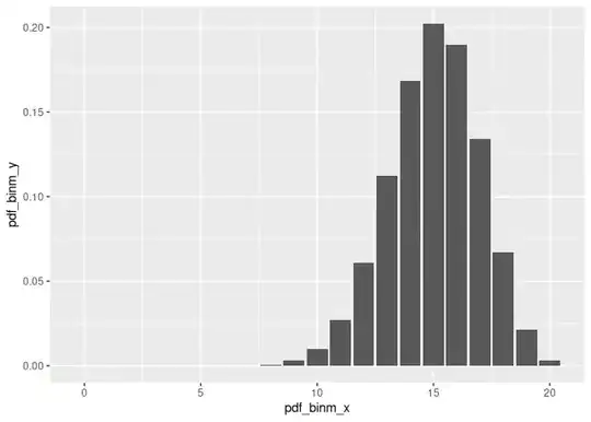
# One single observation from a Binomial distribution
n_trials <- 20
n_successes <- 15
n_failures <- n_trials - n_successes

# MLE of p (rate of success)
p_hat <- n_successes / n_trials

pdf_binm_x <- seq(0, n_trials)
pdf_binm_y <- dbinom(pdf_binm_x, size = n_trials, prob = p_hat)

ggplot(data = data.frame(pdf_binm_x, pdf_binm_y), mapping = aes(x = pdf_binm_x, y = pdf_binm_y)) +
  geom_col()

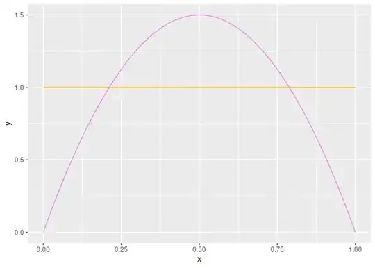
# Flat prior distr.:
beta_prior1_alpha <- 1
beta_prior1_beta <- 1

pdf_beta_x <- seq(0, 1, 0.01)
pdf_beta1_y <- dbeta(pdf_beta_x, shape1 = beta_prior1_alpha, beta_prior1_beta)

# Prior with p around 0.5 more favorable, and decreasing towards 0 and 1.
beta_prior2_alpha <- 2
beta_prior2_beta <- 2
pdf_beta2_y <- dbeta(pdf_beta_x, shape1 = beta_prior2_alpha, beta_prior2_beta)

ggplot(mapping = aes(x = x, y = y)) +
  geom_line(data = data.frame(x = pdf_beta_x, y = pdf_beta1_y), colour = 'orange') +
  geom_line(data = data.frame(x = pdf_beta_x, y = pdf_beta2_y), colour = 'violet')

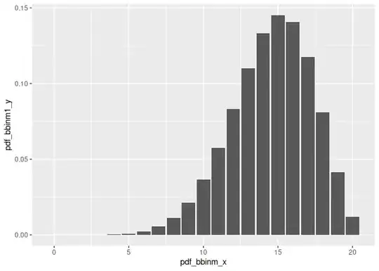
pdf_bbinm_x <- seq(0, n_trials)
pdf_bbinm1_y <- dbbinom(pdf_bbinm_x, size = n_trials, beta_prior1_alpha + n_successes, beta_prior1_beta + n_failures)
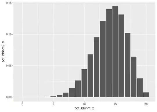
pdf_bbinm2_y <- dbbinom(pdf_bbinm_x, size = n_trials, beta_prior2_alpha + n_successes, beta_prior2_beta + n_failures)

ggplot(data = data.frame(pdf_bbinm_x, pdf_bbinm1_y), mapping = aes(x = pdf_bbinm_x, y = pdf_bbinm1_y)) +
  geom_col()

ggplot(data = data.frame(pdf_bbinm_x, pdf_bbinm2_y), mapping = aes(x = pdf_bbinm_x, y = pdf_bbinm2_y)) +
  geom_col()

^{Created on 2021-10-21 by the reprex package (v2.0.1)}