Estimating growth rate from noisy data?

Question

Let's say we want to estimate growth rate from noisy data. Due to noise, simple calculation will result in very poor estimates (calculating growth rates just exacerbates noise), so smoothing is needed.

This is quite straightforward up to this point, but the question is: how to carry out the smoothing? First smooth the data, and then calculate the growth rate, or the other way around, first calculate the growth rate then smooth these values...?

Here is a small illustration. First, we generate a simulated dataset with a sufficiently complex structure and some noise:

library(ggplot2)
library(data.table)

set.seed(1)

SimData <- data.table(x = 1:501)
SimData$y <- sin(SimData$x/30)
SimData$y <- 200*SimData$y - 0.01*SimData$x^2 + 10*SimData$x + 20
SimData$y <- SimData$y + 50*sin(SimData$x/5)
SimData$TrueGR <- log(SimData$y/c(NA, SimData$y[-nrow(SimData)]))
SimData$y <- round(abs(rnorm(nrow(SimData), SimData$y, 50)) + 1)

plot(SimData$x, SimData$y, type = "l")

Then we try to estimate the growth rate both ways:

SimData$gr <- log(SimData$y/c(NA, SimData$y[-nrow(SimData)]))
SimData <- SimData[-1, ]
SimData$gr1 <- predict(mgcv::gam(gr ~ s(x, k = 50), data = 
                SimData), type = "response")
SimData$SmoothY <- predict(mgcv::gam(y ~ s(x, k = 50), data = 
                SimData, family = mgcv::nb()), type = "response")
SimData$gr2 <- log(SimData$SmoothY/c(NA, 
                SimData$SmoothY[-nrow(SimData)]))
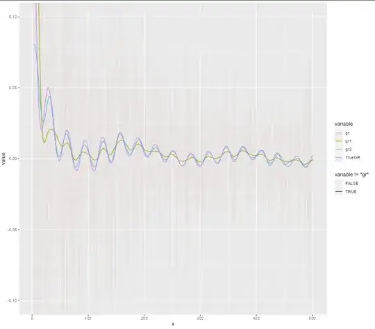
ggplot(melt(SimData[,.(x, gr, gr1, gr2, TrueGR)], id.vars = "x"),
       aes(x = x, y = value, group = variable, color = variable, 
  alpha = variable!="gr")) +
  geom_line() + coord_cartesian(ylim = c(-0.1, 0.1))

It seems that "smooth-first-then-calculate" better picks up the true value, but I don't know whether this is just accidental in this particular example, and a far less know if there is any theory to support either of the approaches.

Answer 1

It makes sense to smooth and then calculate growth rate.

I assume you are interested in the growth rate of the latent measurement (i.e. the noise free value). Smoothing is a method of estimating this latent quantity, and so calculating the growth rate on the smooth is closer to what you want.

Answer 2

I think that the smooth-then-derive method is OK. However there are ways to avoid the 2 steps, I think. For example, one could model the derivative of the trend directly. The idea is the following:

• We observe a series of data $\{x_{i}, y_{i}\}_{i=1}^{n}$ with $y_{i} \sim \mathcal{N}(\mu_{i}, \sigma^{2})$
• $\mu_{i}$ is the $i$th value of a smooth trend function observable at $x_{i}$.
• We are interested in estimating $\dot{\mu} = \displaystyle \frac{d\mu}{dx}$ and the growth rate can be computed as $GR_{i} = \dot{\mu}_{i}/\mu_{i}$ (in the example $dx = 1$...see also below).

In order to solve the estimation task we need the following ingredients (please notice that I tried to keep the notation as simple as possible but might be not perfect):

• A smoother: I will use here P-splines as introduced by Eilers and Marx (1996). P-splines are a class of flexible smoothing techniques combining B-splines and finite difference penalties
• A model for the trend function which will be: $ \hat{\mu} = \displaystyle \int B \alpha $, where $\alpha$ is a vector of unknown spline coefficients to be estimated such that $\hat{\dot{\mu}}= B \hat{\alpha}$ and $B$ is a B-spline matrix built on equally spaced knots.
• Our estimation task then becomes $$ \min_{\alpha} S_{p} = \|y - \int B\alpha\|^{2} + \lambda \|D\alpha\|^{2} $$ where $\lambda$ is a smoothing/regularization parameter and $D$ is a matrix difference operator (I will here use differences of order 2).
• Once we have obtained the $\alpha$ coefficients we can compute $\hat{\mu} = \displaystyle \int B \hat{\alpha}$ and $\hat{\dot{\mu}} = B\hat{\alpha}$.

Below you will find a small code. About the code:

• the integral is approximated with summation
• I use the R-package JOPS to compute the $B$-matrix
• the growth rate is computed 'explicitly' as $(y_{i+1}-y_{i})/y_{i}$
• the fact that the $dx$ is constant and equal to 1 simplifies computations a bit

I left some comments in the code (hope they are clear enough).

library(ggplot2)
library(data.table)
library(JOPS)

set.seed(1)

SimData    = data.table(x = 1:501)
SimData$y  = sin(SimData$x/30)
SimData$y  = 200*SimData$y - 0.01*SimData$x^2 + 10*SimData$x + 20
SimData$sy = SimData$y + 50*sin(SimData$x/5)
SimData$y  = round(abs(rnorm(nrow(SimData), SimData$sy,50)) + 1)

# Extract
x      = SimData$x 
y      = SimData$y
sy     = SimData$sy
TrueGR = c(NA, diff(sy)) / sy # [(i+1)th - ith]/ith

# Integration matrix operator
n  = length(x)
u  = x
Ci = matrix(0, n, n)
for(i in 1:n)
{  
  Ci[i, ] = (x[i] >= u)  
}

# Define bases
bdeg = 3
ndx  = 100
B    = bbase(x, bdeg = bdeg, nseg = ndx) 
nb   = ncol(B)

# Penalty - I fix the lambda parameter (can be selected using e.g. GCV/AIC/BIC etc)
dd = 2
la = 1e1
D  = diff(diag(nb), diff = dd)
P  = crossprod(D) * la

# Smooth
CB    = Ci %*% B 
cof   = solve(crossprod(CB) + P) %*% t(CB) %*% y
mu    = CB %*% cof
dmu   = B %*% cof
hatGR = dmu/mu

# Plot
par(mfrow = c(2, 1), mar = c(2, 2, 2, 2))
plot(x, y, pch = 16, cex = 0.5)
lines(x, y)
lines(x, mu, col = 2, lwd = 2)
lines(x, sy, col = 3, lty = 2, lwd = 2)
legend('topleft', c('Fit', 'Signal'), col = c(2, 3),lty = c(1, 2))

plot(x,  hatGR, col = 2, lwd = 2, type='l',ylim = range(TrueGR, na.rm = TRUE))
lines(x, TrueGR, type = 'l', col = 3, lwd = 2, lty = 2)

The result should look like in the plot below. I hope my answer is clear enough.