Find probability density function of $Y=X^2$ for uniform $X.$

Question

Suppose that a random variable $X$ has a uniform distribution on the interval $[0,1]$. Determine the p.d.f of $X^2$

Following this equation:

$$f(x=y)\frac{dx}{dy}$$

I then solve for $Pr(Y\le y)=Pr(X^2 \le y)=Pr(X\le y^{\frac{1}{2}})$ so that $x=y^{\frac{1}{2}}$

Then taking the derivative of $\sqrt{y}$ I get $\frac{1}{2}y^{-\frac{1}{2}}$

I should get $$y^{\frac{1}{2}}\frac{1}{2}y^{-\frac{1}{2}}=\frac{1}{2}$$

I have taken this from Degroot's Probability and Statistics (third edition- page 164 exercise7.) However the solution is actually $$1 \cdot \frac{1}{2}y^{-\frac{1}{2}} $$

What is the explanation behind this?

Added comments:

$G(y) = Pr(Y \le y) = Pr[r(X) \le y]=Pr[X \le s(y)] = F[s(y)]$

If it is also assumed that s is a differentiable function over the interval $(\alpha, \beta)$, then the distribution of $Y$ will be continuous and the value of its p.d.f $g(y)$ for $\alpha < y < \beta$ will be:

$g(y) = \frac{dG(y)}{dy}=\frac{dF[s(y)]}{dy}=f[s(y)]\frac{ds(y)}{dy}$

In other words, the pdf $g(y)$ of $Y$ can be obtained directly from the pdf $f(x)$ by replacing $x$ but its expression in terms of $y$ and multiplying the result by $dx/dy$

Answer 1

You seem to be mixing two approaches. Instead you should choose one.

Use the CDF, so a density of $f_x(x)=1$ gives $F_X(x)=P(X \le x)=x$ for $0 \le x \le 1$

and so if $Y=X^2$ and $X=Y^{1/2}$

then $F_Y(y) = P(Y \le y)=P(X^2 \le y)=P(X \le y^{1/2}) = y^{1/2}$ for $0 \le y \le 1$

giving a density of $f_Y(y)=F'_Y(y)=\frac{1}{2y^{1/2}}$ for $0 \le y \le 1$.

Or use a change of variables on the density where $f_Y(y) =f_X\big(g^{-1}(y)\big) \left| \frac{d}{dy} \big(g^{-1}(y)\big) \right|$

and here $g(x)=x^2$ and $g^{-1}(y)=y^{1/2}$ which is monotonic for $0 \le y \le 1$,

and $f_X\big(g^{-1}(y)\big)=1$ and $\frac{d}{dy} \big(g^{-1}(y)\big) = \frac{1}{2y^{1/2}}$

so $f_Y(y) =1 \left|\frac{1}{2y^{1/2}} \right| = \frac{1}{2y^{1/2}} $ for $0 \le y \le 1$.

These are the same density, as you might hope.

Answer 2

In the OP's added comments (presumably taken verbatim from Degroot's text), we have that $$g(y) = f(s(y))\frac{\mathrm ds(y)}{\mathrm dy}$$ but the OP's original calculations fail to apply this formula correctly. In the OP's example, $f$ is the uniform density on $[0,1]$ and thus $f(x)$ has value $1$ for all $x \in [0,1]$ The OP correctly calculates $s(y)$ as having value $\sqrt{y}$ and its derivative as $\frac 12 y^{-\frac 12}$ but fails to recognize that $f(s(y))$ has value $1$ whenever the argument $s(y)$ of $f(\cdot)$ is in the interval $[0,1]\,\,$ (and not $y^{\frac 12}$ as he thinks it to be) and so $g(y)$ equals $$\underbrace{~~1~~}_{f(s(y))} \cdot \underbrace{\frac 12 y^{-\frac 12}}_{\frac{\mathrm ds(y)}{\mathrm dy}} = \frac 12 y^{-\frac 12}$$ for $y \in [0,1]$, exactly as Degroot finds it to be, and $\textbf{NOT} ~~y^{\frac 12}\cdot \frac 12 y^{-\frac 12}$ as the OP thinks it to ought to be.

Answer 3

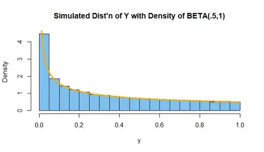
If $F_Y(y) = y^{1/2},$ for $0 < y < 1,$ then $F_Y^\prime (y) = f_Y(y) = \frac 12 y^{-1/2},$ which is the density function of the beta distribution $\mathsf{Beta}(1/2, 1),$ with mean $E(Y) = 1/3.$

Illustration of this 'CDF method' by simulation:

set.seed(812)
x = runif(10^5);  y = x^2
summary(y)
   Min. 1st Qu.  Median    Mean 3rd Qu.    Max. 
0.00000 0.06275 0.24826 0.33192 0.55900 0.99999 

hdr = "Simulated Dist'n of Y with Density of BETA(.5,1)"
hist(y, prob=T, br=30, col="skyblue2", main=hdr)
 curve(dbeta(x, .5, 1), add=T, lwd = 3, col="orange")

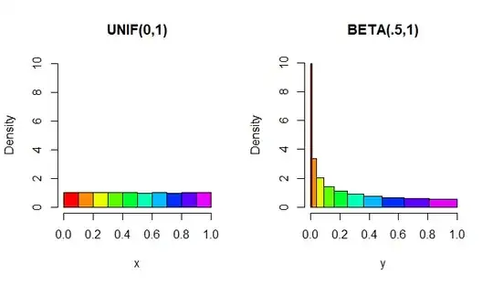
Addendum: In the histograms below, images and objects of the transformation are represented by bars of the same color; all bars have (very nearly) the same area. [In the 'PDF method', the shape of the beta histogram arises from $dx/dy.]$

set.seed(2021)
x = runif(10^5);  y = x^2
cutp = seq(0,1,by=.1)
par(mfrow=c(1,2))
 hist(x, prob=T, br=cutp, ylim=c(0,10), col=rainbow(11), main="UNIF(0,1)")
 hist(y, prob=T, br=cutp^2, col=rainbow(11), main="BETA(.5,1)")
par(mfrow=c(1,1))