3

If the beta distribution is a prior of a Bernoulli distribution (i.e. a rate of success for a binary outcome), then it is completely counterintuitive to me that the beta distribution should be equivalent to the uniform distribution when a, b = 1.

Unless I'm mistaken, you can interpret a and b to be the number of measured successes and failures of your outcome (e.g. heads or tails of a flipped coin). If that's true, then the likelihood of your posterior Bernoulli parameter being either 0 or 1 should be much closer to 0 (i.e. and NOT equally likely as values closer to 0.5).

If the underlying Bernoulli really was as likely to be 0 or 1 as something closer to 0.5, you would NOT expect to get both a 0 and a 1 out of two samples, right?

What am I missing that would make this more intuitive?

  • 3
    "If the underlying Bernoulli really was as likely to be 0 or 1 as something closer to 0.5, you would NOT expect to get both a 0 and a 1 out of two samples, right?" This suggests a beta-binomial model for $a=b=1$, which is a discrete uniform variable. There doesn't seem to be a contradiction. – Sycorax Jul 09 '21 at 21:05
  • 5
    You seek intuition. One place is the discussion at https://stats.stackexchange.com/questions/4659. Another is to study Bayes' billiard table experiment (Google it). The case $a=b=1$ corresponds to the situation after a single ball has been rolled on the table: it could be anywhere, with constant probability density. That's the uniform distribution. – whuber Jul 09 '21 at 21:35
  • [Non-informative priors do not exist!](https://stats.stackexchange.com/a/249752/7224) – Xi'an Jul 10 '21 at 12:37
  • The interpretation of $a$ and $b$ being the number of (virtual) successes and failures observed a priori is a way to calibrate and understand the prior, no a real thing, especially when $a$ or $b$ are less than one. – Xi'an Jul 10 '21 at 12:40

2 Answers2

2

Every conjugate prior distribution to an exponential family has some set of parameters $\eta_0$ that result in a uniform distribution over the space. You can see this here by considering what happens to the natural parameters $\eta'$ of the conjugate prior when the number of pseudo-observations $n$ equals $0$.

Unless I'm mistaken, you can interpret a and b to be the number of measured successes and failures of your outcome (e.g. heads or tails of a flipped coin). If that's true, then the likelihood of your posterior Bernoulli parameter being either 0 or 1 should be much closer to 0 (i.e. and NOT equally likely as values closer to 0.5).

That is true, but beta$(1, 1)$ corresponds to $a=b=0$. The natural parametrization of the beta distribution is $(\alpha-1, \beta-1)$ compared the "source parametrization" (or common parametrization) of $(\alpha, \beta)$.

Neil G
  • 13,633
  • 3
  • 41
  • 84
1

In Bayesian statistics one uses a 'flat' prior distribution for a parameter in the absence of knowledge or opinion about about 
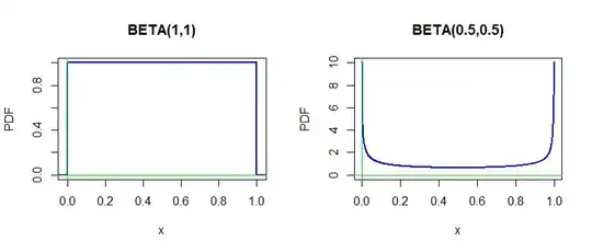
the parameter value. When the parameter is binomial success probability $p$ it may seem natural to use either a uniform prior $\mathsf{Beta}(\alpha=1,\beta=1)\equiv\mathsf{Unif}(0,1)$ or even the "bathtub shaped" prior $\mathsf{Beta}(.5, .5).$

enter image description here

par(mfrow=c(1,2))
 hdr1 = "BETA(1,1)"
 curve(dbeta(x,1,1), -.05,1.05, ylab="PDF", 
   col="blue", lwd=2, xaxs="i", n=10001, main=hdr1)
  abline(v=0, col="green2"); abline(h=0, col="green2")
 hdr2 = "BETA(0.5,0.5)"
 curve(dbeta(x,.5,.5), 0,1, ylab="PDF", col="blue", lwd=2, 
   ylim=c(0,10), n=1001, main=hdr2)
  abline(v=0, col="green2"); abline(h=0, col="green2")
par(mfrow=c(1,1))

The purpose of using a flat prior distribution may be for the posterior distribution on the parameter to be mainly due to the data. For example, if the prior is $\mathsf{Beta}(1,1)$ and the data show $x=23$ successes in $n=50$ trials, then the likelihood is proportional to $p^x(1-p)^{n-x} = p^{23}(1-p)^{27}.$

Thus the posterior distribution is $\mathsf{Beta}(24, 28)$ and a 95% Bayesian credible interval for $p$ is $(0.33,\,0.600,$ which agrees numerically with a frequentist 95% frequentist Agresti-Coull confidence interval $(0.33,\,0.60)$ to two decimal places.

qbeta(c(.025,.975),24,28) 
[1] 0.3293001 0.5965812
p.est = 25/54
p.est + qnorm(c(.025,.975))*sqrt( p.est*(1-p.est)/54 )
[1] 0.3299707 0.5959553

Note: The distribution $\mathsf{Beta}(.5,.5)$ is called a Jeffreys prior. It can be argued that it is less informative as a prior than is $\mathsf{Beta}(1,1).$ The interval estimate $(0.33, 0.60)$ from this prior distribution is sometimes used as a frequentist CI:

qbeta(c(.025,.975),23.5,27.5) 
[1] 0.3273505 0.5971336
BruceET
  • 47,896
  • 2
  • 28
  • 76
  • 2
    "In Bayesian statistics one uses a 'flat' prior distribution for a parameter in the absence of knowledge or opinion about about the parameter value." Sorry, but I think it's a common mistake to consider a flat prior to be uninformative. Any prior to some distribution $D$ can be made flat by simply reparametrizing $D$. – Neil G Jul 10 '21 at 07:03
  • 1
    I agree that a flat likelihood is uninformative though. – Neil G Jul 10 '21 at 07:09