0

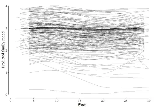
I have a problem with two forms of plots of two GAMM models: The first model is a baseline model estimating the time trend of measured mood during 30 weeks of 2020 (N=371). Lot's of missings, though (but I hope I can deal with that with a GAMM). The results for the first model show the best fit for a random smooth model:

Parametric coefficients:
            Estimate Std. Error t value Pr(>|t|)    
(Intercept)  2.69041    0.03282   81.97   <2e-16 ***
---
Signif. codes:  0 ‘***’ 0.001 ‘**’ 0.01 ‘*’ 0.05 ‘.’ 0.1 ‘ ’ 1

Approximate significance of smooth terms:
                 edf   Ref.df     F  p-value    
s(x)           5.014    6.254 4.505 0.000118 ***
s(x,user_id) 550.871 1623.000 3.466  < 2e-16 ***

In the summary, x is the time variables (t = 1 to 30) and s(x,user_id) is the random smooth. When I use the predict() function and plot the individual trends with ggplot, I get a picture of almost non-changing trends with a slight non-linearity (mood went down in fall 2020 and stayed there). However, some individuals started low and had a decline (5% of the sample). Baseline random smooth plot
The next progression in the model building is an interaction between time and self-reported health (mhem1_r) which turns out to be significant:

Approximate significance of smooth terms:
                  edf   Ref.df      F  p-value    
s(x)            5.068    6.317  4.365 0.000162 ***
s(x,user_id)  539.803 1623.000  2.830  < 2e-16 ***
s(mhem1_r)      1.827    1.876 51.953  < 2e-16 ***
ti(x,mhem1_r)  10.829   88.000  0.224 0.001788 ** 

When I use vis.gam() to get a 3D surface plot, three really weird things happen:

enter image description here

  1. The whole level of the surface is too low and differs from the baseline plot (which the intercepts in the output show).
  2. The trend looks so different: Whereas in the baseline plot, mood was rather stable, the vis.gam plot shows a downward trend followed by an upward trend.
  3. I really cannot see any interaction....
  4. A final thing: Although the main effect and interactions of/with perceived health are signficant, the R-sq is almost the same (.631 vs. .634) in both models.

Has anybody an idea what the problem is?

All the best and thank you in advance :)

Holger

P.S. Here is the code for both models in case this is the source of error

#Baseline model
gamm2c <- bam(mood ~ s(x, bs="cr", k=30) +
                       s(x, user_id, bs="fs", xt="cr", m=1, k=5)+
                      data=weekly_data, method="fREML")

#Interaction model
gamm_mhem <- bam(mood ~ s(x, bs="cr", k=30) +
                        s(x, user_id, bs="fs", xt="cr", m=1, k=5)+
                        s(mhem1_r, bs="cr", k=5) +
                        ti(x, mhem1_r, bs="cr", k = c(30,5)), 
                        data=weekly_data, method="fREML")
  • I'm not sure I understand the problem. You changed the model fairly substantially and it now shows you a somewhat different pattern. That's a fairly common occurrence, especially with a flexible model like a GAMM. I don't know how it's possible for us to judge that "The whole level of the surface is too low". – mkt Jul 05 '21 at 12:13
  • Hi, thanks for the comment. With regard to the first problem, the baseline plot shows that the majority of trends are in the area between 2 and 4 whereas in the interaction plot, the surface is below 2 (doesn't fit with the intercept of 2.69 in the baseline model. Isn't that weird? With regard to the differences in the models: I simple added a predictor but that should not lead to different trends, do they? When the baseline model shows that not many persons went upwards again, how does that change a predictor? If this not weird, I am happy. :) – HolgerSteinmetz Jul 05 '21 at 12:42
  • 1
    (i) You are ignoring the random effects in the plot with interaction, and (ii) it's below 2 only at low values of mhem1_r; it looks like it is above 2 when mhem1_r is high. – mkt Jul 05 '21 at 13:05
  • `I simple added a predictor but that should not lead to different trends, do they?` This happens all the time, actually. And is a common problem when doing model selection and interpreting models. – mkt Jul 05 '21 at 13:05
  • e.g. https://stats.stackexchange.com/questions/1580/regression-coefficients-that-flip-sign-after-including-other-predictors – mkt Jul 05 '21 at 13:07
  • 1
    Thank you so much! Yes that makes perfect sense: Mhem is highly skewed, so the majority of the sample is a that "higher side" of mood. All the best, Holger – HolgerSteinmetz Jul 05 '21 at 13:23
  • You should transform `mhem` then (assuming you haven't already) to spread the data out otherwise the entire spline will be mostly determined by the few large values because the knots are spread out evenly through the range of the covariate. – Gavin Simpson Jul 05 '21 at 15:05
  • Also, `vis.gam` will set the other variables in the model that you're not plotting to some reference level. I forget exactly what it does with factors (the modal level IIRC) but it will be showing you the response for one of your `user_id`s, which is likely why the surface is lower than you expect; it could easily have used one of the levels that is towards the bottom of the first figure... – Gavin Simpson Jul 05 '21 at 15:07
  • Dear @GavinSimpson thank you (as so often) for your comment: 1) Transforming did not change the results. 2) Your second comment however puzzles me a bit. Does that mean that vis.gam cannot be used to show the shape of the overall interaction? Do you haven idea where to find some background what the function does when having random effects? All the best, Holger – HolgerSteinmetz Jul 06 '21 at 11:36
  • 1
    Re 2: `vis.gam()` takes the two specified covariates and constructs a grid of points over the range of each covariate, crosses them so you get a grid over combinations of the two covariates, then calls `predict.gam()` on those values to get predicted values for those covariate combinations. As `predict.gam` requires values for all other covariates in the model, unless you tell it differently it will choose the modal level for each factor variable and the data observation closest to the mean (or median, I forget) of each covariate in the observed data. These are then constant over the grid. – Gavin Simpson Jul 06 '21 at 18:34
  • 1
    As a random effect or random factor smooths, these are seen by `gam` as smooths, they follow the same behaviour as described above. You can exclude terms using `exclude`; create a character vector with the smooths you want to exclude, using the names as given in the output from `summary()`. Note that you still have to provide some values for all covariates, even if they end up being excluded; `vis.gam` arranges this for you. Plotting the `ti()` term will show the interaction, but I suspect you meant the combination of marginal smooths plus `ti`, in which case I would... – Gavin Simpson Jul 06 '21 at 18:38
  • 1
    ...start with creating data for predicting at, use `predict` (ignore what I said about `vis.gam` and `exclude` - it isn't an option, just in `predict` so you're doing everything by hand), and then `exclude` all the terms you aren't interest in, or more easily use `terms` argument to select on the three you need `terms = c("s(x)", "s(mhem1_r)", "ti(x,mhem1_r)")`, which will give you predicted values but only including the contributions from those three terms (plus the intercept). If you want more control, use `type = "terms"` and sum over the columns you want to include in the fitted values – Gavin Simpson Jul 06 '21 at 18:45

0 Answers0