Interpreting bootstrap CIs

Question

Are central values in a bootstrap confidence interval more likely for the population parameter concerned than the values near the boundaries? This interpretation applies to parametric CIs but does it apply to bootstrap CIs also? Thanks!

Answer 1

You'd have to be careful what you mean by more likely.

To make a traditional z interval with confidence $1-\alpha$ for normal mean $\mu$ $(\sigma$ known), you can begin with $P\left(\frac{\sigma}{\sqrt{n}}L <\bar X - \mu<\frac{\sigma}{\sqrt{n}}U\right),$ where $L$ and $U$ cut probability $\alpha/2$ from the lower and upper tails of standard normal distribution. So the highest density (likelihood) is between $L$ and $U.$ Then 'pivot' to get the $1-\alpha$ CI $\left( \bar X- \frac{\sigma}{\sqrt{n}}U,\; \bar X -\frac{\sigma}{\sqrt{n}}L \right)$ for $\mu.$ But be careful with the terminology: A 90% CI is shorter than a 95% interval,

Similarly, if I am making a $1-\alpha$ nonparametric quantile bootstrap CI for $\mu$ for a sample from a distribution with mean $\mu,$ but unknown shape, I will re-sample of many values $\bar X^*$ (a.re in the R code) based on re-samples of size $n$ with replacement from my sample x of $n$ observations from such a population.

Consider the sample with numerical and graphical summaries below.

summary(x);  length(x);  sd(x)
   Min. 1st Qu.  Median    Mean 3rd Qu.    Max. 
  29.31   61.85   69.10   67.71   75.80  106.72 
[1] 50         # sample size
[1] 13.87644   # sample SD

boxplot(x, col="skyblue2", pch=20, horizontal=T)

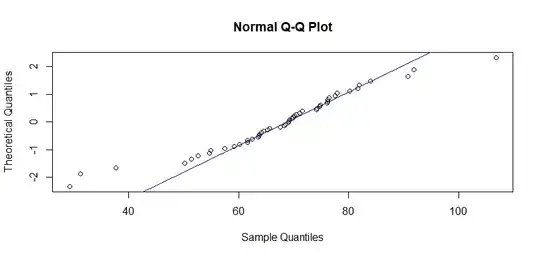
The data are pretty clearly not normal: Their normal probability plot is distinctly non-linear, and a Shapiro-Wilk test rejects normality.

shapiro.test(x)$p.val
[1] 0.03938396
qqnorm(x, datax=T);  qqline(x, datax=T, col="blue")

So, I decide against a t confidence interval, in favor of a bootstrap CI for $\mu,$ which has point estimate $\bar X = 67.71.$

A basic 95% quantile nonparametric bootstrap Ci $(63.8.\, 71.5)$ is obtained as shown below. [Bootstrap resampling is a random process, so results may differ slightly among runs, if you use a different seed (nor none). Three additional runs gave $(63.4, 71,4),$ $(63.7, 71.6),$ and $(63.6, 71.6).]$

set.seed(701)
a.re = replicate(3000, mean(sample(x, 50, rep=T)))
CI = quantile(a.re, c(.025, .975));  CI
     2.5%    97.5% 
 63.84828 71.50980 

The bootstrap distribution of re-sampled means is shown below, along with vertical lines for the confidence limits. The most commonly occurring resample averages are between the confidence limits, and near the point estimate $\bar X = 67.71.$ (For other, more sophisticated types of bootstrap CIs, similar arguments might be made that, in some sense, the "most likely" possible values of $\mu$ lie near the center of the CI.)

hist(a.re, prob=T, col="skyblue2")
 abline(v = CI, col="red", lwd=2, lty="dotted")

---

Notes: The data x used above was sampled in R from a Laplace distribution as follows:

set.seed(2021)
x = rexp(50, .1) - rexp(50, .1) + 70

Although I wouldn't have wanted to rely on it, the legendary robustness of t methods is evident here: A t confidence interval for $\mu$ is $(63.8, 71,7);$ not much different from the bootstrap CI above. [In this case with fictitious simulated data the 95% nonparametric CI does happen to contain the population mean $\mu = 70.$ Of course, in most real applications one never knows the true value of $\mu.$]

t.test(x)$conf.int
[1] 63.76484 71.65212
attr(,"conf.level")
[1] 0.95