Statements in your Question seem to be on the right track. Congratulations on getting that part right. But there is more. Here are some
comments on closely related topics for you to consider.
When using a t test for a two-sided alternative (for example
$H_0: \mu = 100$ against $H_a: \mu \ne 100),$ at the level $\alpha = 0.05 = 5\%,$ the critical
values are set to cut 2.5% of the area under the appropriate
t distribution from each tail of the distribution.
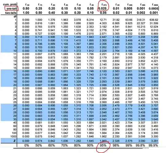
For example, if DF = 24, then critical values are $c = \pm 2.064$ from your table, so that you reject if the $T$ statistic has
either $T \le -2.064$ or $T \ge 2.064.$ Usually, this is
combined into one statement that you reject if $|T| \ge 2.064.$
In R, $c=2.064$ for the upper tail can be found as follows, then you can find the lower-tail critical value using the symmetry a t distribution about $0.$
[In R, qt is the quantile function, which finds the t-value with the designated probability below it; many printed t tails show 'percentage points', with the desired
probability above. Notice that your table uses the notation
$t_{24; .975} = 2.064,$ but the bold headers have probabilities above the tabled value.]
qt(.975, 24)
[1] 2.063899
qt(.025, 24)
[1] -2.063899
Now consider a normal sample x of size $n = 25$ from a normal
distribution. It has sample mean $\bar X = 107.14, S = 16.98.$
set.seed(2021)
x = rnorm(25, 104, 15)
summary(x);  length(x);  sd(x)
   Min. 1st Qu.  Median    Mean 3rd Qu.    Max.
  75.16   99.91  107.93  107.14  122.12  129.95
[1] 25
[1] 16.98381
In R, a t test of $H_0: \mu = 100$ against $H_a: \mu \ne 100$
is shown below:
t.test(x, mu=100)

        One Sample t-test

data:  x
t = 2.1025, df = 24, p-value = 0.04618
alternative hypothesis: true mean is not equal to 100
95 percent confidence interval:
 100.1313 114.1524
sample estimates:
mean of x
 107.1418
If we use the information from the discussion above, we know
that we reject $H_0$ (just barely) because $T = 2.1025$ (rounded from $2.102539)$
has $|T| = 2.1025 > 2.06.$ (Notice that the printed value of $T$ is rounded from $2.102539.)$
By contrast, if we use the information in the R output, we
know to reject $H_0$ because the two-sided test has P-value
$0.04618 \le 0.05 = 5\%.$ The P-value is the area under the
density curve of Student's t distribution with DF = 25,
the is either below $-2.1025$ or above $2.1025.$
The P-value can be computed in R (where pt is the CDF of a t distribution) as shown below.
B = pt(-2.1025, 24);  B
[1] 0.02309119
A = 1 - pt(2.1025, 24);  A
[1] 0.02309119
A + B
[1] 0.04618239
In the figure below the critical values are at vertical lines, cutting 0.025 from each
tail of the distribution $\mathsf{T}(\nu = 24),$ are shown in red,
the observed $T$ in solid blue. The P-value is the total
area under the density curve outside the two blue lines.

R code for figure:
hdr = "Density of T(24) with 5% two-sided critical values (red)"
curve(dt(x, 24), -4, 4, lwd=2, ylab="PDF", xlab="t", main=hdr)
 abline(h = 0, col="green2")
 abline(v = 0, col="green2")
 abline(v = c(-2.064, 2.064), lwd=2, col="red")
 abline(v = 2.1025, col="blue", lwd = 2)
 abline(v = -2.1025, col="blue", lwd=2, lty="dotted")
Note: Unless you use a parameter for a different confidence
level, the R output of t.test gives a 95% confidence interval
for the population mean $\mu.$
Because the data came from
simulation we know that $\mu = 104$ happens to lie within the given CI
$(100.1313, 114.1524).$ In a real application, one never knows
the exact value of $\mu.$
 As far as I know for two tail we will split