How to explain the coefficient plotting as pre-trend stability testing for generalized Difference-in-Differences?

Question

Proving the pre-trend parallel is hard in generalized DiD. From this post, Thomas Bilach suggests me a very excellent way to do so which is called "coefficient plotting"

In short, it can be achieved by running this equation

$$y_{kt} = \alpha_k + \lambda_t + \delta_{-2} d_{k,t-2} + \delta_{-1} d_{k,t-1} + \delta d_{kt} + \delta_{+1} d_{k,t+1} + \delta_{+2} d_{k,t+2} + \delta_{+\bar{3}} d_{k,t+\bar{3}} + \epsilon_{kt}$$

And then, we will see "how close the $\delta$ to 0" for pre-trend periods if I understand correctly. Some examples can be seen in the answer of @Thomas Bilach above.

My effort is that I try to mimic what @Thomas Bilach suggests, along with adding some more covariates (independent variables). However, my result is as below, which make me feel hard in explaining regarding "how close to 0"

For example, I run such regression for two different dependent variables called $y1_{kt}$ $y2_{kt}$

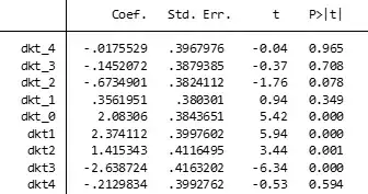
The results for is $y1_{kt}$

While dkt_4 is $d_{k,t-4}$, dkt4 is $d_{k,t+4}$ As can be seen, p-value of dkt1 is higher than 0.1, insignificant, so whether we still plot the coefficient even it is insignificant.

Apart from that, from the result above, is there any conclusion about the impact of laws on the dependent variable $y1_{kt}$ why the lead indicators seem to be smaller than that of lad indicators?

The result for $y2_{kt}$

How can we explain the stability trend in this case?

Answer 1

A quick word with respect to the "naming" of your variables. First, the only thing separating the lead variables from the lag variables is an underscore (e.g., _). This makes reviewing your output very confusing. I would imagine it's difficult for you as well, especially when returning to your project after a brief hiatus. Thus, I recommend generating 'event study' variables that you can easily recognize (e.g., lead_3, lead_2, lead_1). The same applies to your lags (e.g., lag_0, lag_1, lag_2). In short, I should be able to distinguish the pre/post epoch instantaneously.

Second, what is dkt_0 denote? Is it the last pre-treatment period or the immediate adoption period (i.e., year of change)? The _ suggests it's a lead, however the numeric value appended to it suggests it's the first adoption year. Going forward I will assume dkt_0 is the immediate adoption year, with dkt1 serving as the first lag.

In the first table, the lead coefficients suggest a deviation from a common trend. The difference appears to stabilize by the second lag, but not for long. Thus, your set of coefficients for the outcome $y^{1}_{kt}$ suggest rather strong pre-trends, which casts doubt on the assumption of trend equivalence before policy adoption. On the other hand, the second table is bit closer to what we would expect to see in a traditional 'event study' framework. The leads suggest a stability of the trends across units in the epoch before the policy change, with a positive treatment effect emerging in the year of change. Effects persist in subsequent periods.

Lastly, ignoring the early post-treatment effects simply because they bound zero is very suspicious. If we don't discover punctual change, it could be that effects emerge with a lag! A discovery of a delayed effect may be of substantive interest. Conversely, dropping insignificant downstream effects may fail to show when the effects of a policy dissipate. In sum, we can't reliably exploit when policy effects phase-in (phase-out) if you only report a subset of highly significant post-treatment effects. Thus, never do this.

Remember, we typically plot the coefficients to show their evolution over time, so it's important that we preserve the chronology of effects within the event window—regardless of their significance. A finding of an insignificant program/policy effect may be, in and of itself, a significant discovery.