I am confused by the visualizations of the likelihood, prior and posterior distribution that I usually see when the Bayes' theorem is explained. An example is the image below:
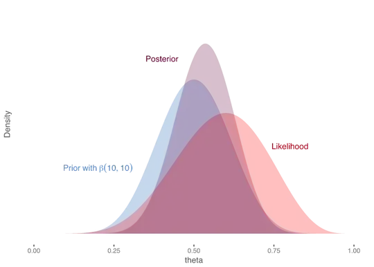
The x-axis shows the parameter $\theta$ and the y-axis represents the density. The definition of the distributions is the following:
Likelihood = P(Data | $\theta$)
Prior = P($\theta$)
Posterior = P($\theta$ | Data)
Given these definitions, I understand the Prior and Posterior plot (since we are visualizing the distribution of the parameters), but the plot of the likelihood distribution shown above is trickier. I understand the plot of the likelihood distribution where the x-axis shows the data. In the case shown above, if we assume that: (1) the likelihood = 0.8 when $\theta$ = 0.5, (2) the likelihood is Normally distributed and (3) the data is i.i.d, is it correct to say the following?
$$ \prod_i^N \mathcal{N}(x_i \ \ | \ \ \theta=0.5, \sigma) = 0.8$$