What is an intuitive explanation for Q90 (X+Y) > Q90(X) + Q90(Y) in fat-tailed variables. Non Subadditivity

Question

In a business situation, management keeps a reserve of money for a 'rainy day' just in case costs are more than expected. The 90th percentile ($Q_{90}$ in the following) might be an indicator of how much costs might reach in adverse conditions.

If I have two such costs, completely independent, I would expect that $$Q_{90}(X+Y)<Q_{90}(X)+Q_{90}(Y)$$ That is, if I hold enough reserve for each risk, it should certainly be enough for the sum: adding risks together usually entails some diversification benefit.

But in my case, this does not hold.

How can I intuitively understand this?

To give a specific example:

let $X\sim \operatorname{lognormal}(0,3)$ and $Y\sim\operatorname{lognormal}(0,3)$ They are completely independent.

From simple sampling in Excel (10k simulations), I get:

$$Q_{90}(X)=Q_{90}(Y)\approx 45$$ $$Q_{90}(X)+Q_{90}(Y)=90$$ but $$Q_{90}(X+Y)\approx 138$$

Answer 1

TLDR; Let's define $Q_X(0.9) = c$ as the reserved costs. And $2c$ will be the costs reserved for two variables $X$ and $Y$.

For the specific case in the question, the probability for $X+Y$ to exceed $2c$ is larger than 10%, namely 13.16%.

This is because the probability for $X$ and $Y$ to exceed $2c$ is already individually more than 5%, namely 6.52%.

When $X$ and $Y$ are independent then the probability for the sum $X+Y>2c$ is larger than the sum of probabilities $X>2c$ and $Y>2c$.

---

A sufficient condition for $Q_{X+Y}(0.9)> Q_X(0.9) + Q_Y(0.9)$ can be expressed in terms of the survival function.

Note that

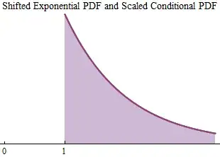
• There is an equivalent statement in terms of quantile functions and survival functions $$Q_{X+Y}(0.9)> 2c \quad \equiv \quad S_{X+Y}(2c) > 0.1$$ Note the blue arrows in the image below. Vertical arrow: The survival function of $X+Y$ in the point $2c$ is above $0.1$. Horizontal arrow: The 0.9 quantile of $X+Y$ is above $2c$.

• The survival function of a sum is larger than the sum of the survival functions. $$S_{X+Y}(2c) \geq S_X(2c) + S_Y(2c)$$ This is because $X+Y$ is larger than $2c$ when either $X$ or $Y$ is larger than $2c$

So a sufficient condition for $Q_{X+Y}(0.9)> Q_X(0.9) + Q_Y(0.9)$ is when

$$S_{X}(2c) > \frac{S_{X}(c)}{2}$$

where $c = Q_X(0.9) = Q_Y(0.9)$. This is because if $S_X(2c)$ is larger than half the $S_X(c)$, then $S_{X+Y}(2c)$ (which is at least twice $S_X(2c)$) will be larger than $S_X(c)$ and this is equivalent to the 0.9-th quantile being larger than $2c$

---

Relationship with tails.

For distributions where the survival function approaches a power law

$$S(x) = Pr[X>x] \sim x^{-\alpha}$$

The condition $Pr[X>2x] > Pr[X>x]/2$ will be fulfilled if $\alpha < 1$.

This condition does not relate to just any distribution with heavy tails. the cases with $\alpha < 1$ have an infinite or undefined mean.

So the case with the lognormal distribution, which does not approach a power-law tail, is not a property of the tails. It happens because in the beginning close to $0$ the survival function will fall less quickly then $1/x$, but in the tails, this is not the case anymore.

See the image below where the distribution of $2X$ and $X+Y$ is compared in terms of the survival function. At some point the survival function of $X+Y$ is below the survival function of $2X$, this is also the point where no more the property for the quantile function is true.

In the image, we plotted gray broken lines that relate to the $\propto 1/x$ relationship. The point where the two survival functions cross is also where the slope becomes steeper than the $1/x$ relationship.

Answer 2

This is a visual answer: a careful consideration of the second figure shows what is going on. Everything else in this post is only a gloss on that figure.

---

In this figure of the $(x,y)$ plane, region $I$ (blue, top) consists of all $y$ values exceeding a quantile $Q_{90}(Y),$ region $II$ (red, right) consists of all $x$ values exceeding a quantile $Q_{90}(X),$ and therefore their intersection (purple, top right) shows all points $(x,y)$ where both $x\ge Q_{90}(X)$ and $y \ge Q_{90}(Y).$

This figure has been drawn to scale, so that the line $x+y=Q_{90}(X)+Q_{90}(Y)$ will make an angle of $-45$ degrees, it will pass through the central point $(Q_{90}(X), Q_{90}(Y)),$ and all points $(x,y)$ whose sum exceeds this threshold will lie to the upper right of that line:

The question wonders about the circumstances that would permit the probability of the combined three regions $B\cup C \cup D$ to exceed $100\%-90\%,$ for then the $90^\text{th}$ quantile of $X+Y$ would have to lie even further above and to the right.

This way of reframing the question makes the answer generally clear, whether or not $X$ and $Y$ are independent: we need only concentrate most of the probability from regions $I\cup II,$ as colored in the first figure, within the three regions $B\cup C\cup D$ (that green triangle in the second figure).

When $X$ and $Y$ are independent it's a little tricky to do that, because independence implies $$\Pr(C) = \Pr(I\cap II) = \Pr(I)\Pr(II) = (1-0.9)(1-0.9) = 0.01,$$ severely limiting how much probability we can assign to $C.$ Observe, though, that including $B$ and $D$ can greatly increase the probability of $B\cup C\cup D.$ If we make sure most of the probability of the events $I$ and $II$ is located way above and way to the right (respectively), then $B \cup C$ can include almost all of the probability of $I.$ That is, we can make $\Pr(B\cup C) \le 1 - 0.9=0.1$ arbitrarily close to $0.1$ and likewise we can make $\Pr(D\cup C)$ arbitrarily close to $0.1.$ Consequently we obtain the bounds, which clearly can be approached as nearly as we might desire, of

$$\Pr(B\cup C\cup D) = \Pr(B\cup C) + \Pr(D\cup C) - \Pr(C) \le 0.1 + 0.1 - 0.01 = 0.19.$$

These considerations lead immediately to a simple example: let's put atoms at appropriate places within the figure. For instance, at the places where the symbols "A" through "E" are drawn, assign concentrated probabilities symmetrically in $x$ and $y$ as follows by choosing an arbitrarily tiny positive $\epsilon:$

$$\cases{A: 0 \\ B: 1-0.9-\epsilon\approx 0.1 \\ C: (1-0.9)^2=0.01 \\ D: 1-0.9-\epsilon\approx 0.1 \\E: 0}$$

and distribute the rest of the probability to the left and below everything else, again symmetrically, so that $X$ and $Y$ have identical and independent distributions.

Notice this says almost nothing about how heavy the tail of this common distribution might be! In the example, this distribution could have an upper limit just barely greater than $Q_{90}.$

Answer 3

As distributions get more right-tailed, the $90^{th}$ percentile of $X+Y$ approaches the $\frac{3}{\sqrt{10}}$th quantile of $X$, roughly the $95^{th}$ percentile. In other words, the top 10% of combined losses will come from roughly 5% in which the first loss is as high as possible, and 5% in which the second loss is as high as possible. (The number $3/\sqrt{10}\simeq.9487$ is a more exact limit which avoids double-counting when both $X$ and $Y$ are high.) So the counterintuitive situation in the post will arise whenever $Q_{95}(X)\gg2Q_{90}(X)$, which is the case with $LN(0,3)$.

Here is an analogous situation where the math is simpler.

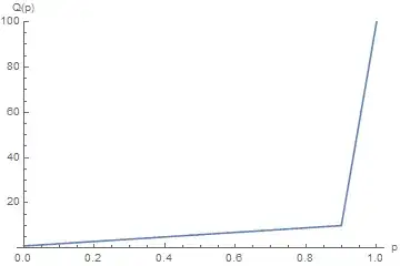
Suppose 90% of the losses are uniformly distributed between 1 and 10, and 10% of the losses are uniformly distributed between 10 and 100. Then

$$Q_{90}(X)=10,\ \, Q_{95}(X)=55,\ \ Q_{90}(X+Y)\simeq 60$$

The quantile function for $X$ has an especially simple form: $$Q_p(X)=\begin{cases} \ \ 10p+1\quad\ \text{ if }\ \ 0.0<p<0.9\\ 900p-800\ \text{ if }\ \ 0.9<p<1.0\\ \end{cases}$$

The graph below shows the percentile for the first loss on the $x-$axis, the percentile for the second loss on the $y-$axis, and the blue region where the sum of the two losses is less than 60, i.e. $Q_p(X)+Q_q(Y)<60$:

The blue region has 90% of the area of the square, which is 90% of the probability. It intersects the axes near 0.95, leaving out roughly 5% of the square on top and 5% of the square on the right, corresponding to the 5% highest $X$ and $Y$.

Answer 4

Using the business world example: Quantile measures of risk exclude worst-case scenarios. When a distribution is very fat-tailed, a measure such as $Q_{90}$ will exclude almost all bad scenarios and deceptively present an innocent-looking risk.

But when risks are summed, we are now looking at the risk of at-least-one-bad-thing-happening. The more risks, the higher the chance that at least one thing will go wrong, and the higher the risk reserve for a rainy day that must be carried.