Empirical distribution alternative

Question

BOUNTY:

The full bounty will be awarded to someone who provides a reference to any published paper which uses or mentions the estimator $\tilde{F}$ below.

Motivation:

This section is probably not important to you and I suspect it won't help you get the bounty, but since someone asked about the motivation, here's what I'm working on.

I am working on a statistical graph theory problem. The standard dense graph limiting object $W : [0,1]^2 \to [0,1]$ is a symmetric function in the sense that $W(u,v) = W(v,u)$. Sampling a graph on $n$ vertices can be thought of as sampling $n$ uniform values on the unit interval ($U_i$ for $i = 1, \dots, n$) and then the probability of an edge $(i,j)$ is $W(U_i, U_j)$. Let the resulting adjacency matrix be called $A$.

We can treat $W$ as a density $f = W / \iint W$ supposing that $\iint W > 0$. If we estimate $f$ based on $A$ without any constraints to $f$, then we cannot get a consistent estimate. I found an interesting result about consistently estimating $f$ when $f$ comes from a constrained set of possible functions. From this estimator and $\sum A$, we can estimate $W$.

Unfortunately, the method that I found shows consistency when we sample from the distribution with density $f$. The way $A$ is constructed requires that I sample a grid of points (as opposed to taking draws from the original $f$). In this stats.SE question, I'm asking for the 1 dimensional (simpler) problem of what happens when we can only sample sample Bernoullis on a grid like this rather than actually sampling from the distribution directly.

references for graph limits:

L. Lovasz and B. Szegedy. Limits of dense graph sequences (arxiv).

C. Borgs, J. Chayes, L. Lovasz, V. Sos, and K. Vesztergombi. Convergent sequences of dense graphs i: Subgraph frequencies, metric properties and testing. (arxiv).

Notation:

Consider a continuous distribution with cdf $F$ and pdf $f$ which has a positive support on the interval $[0,1]$. Suppose $f$ has no pointmass, $F$ is everywhere differentiable, and also that $\sup_{z \in [0,1]} f(z) = c < \infty$ is the supremum of $f$ on the interval $[0,1]$. Let $X \sim F$ mean that the random variable $X$ is sampled from the distribution $F$. $U_i$ are iid uniform random variables on $[0,1]$.

Problem set up:

Often, we can let $X_1, \dots, X_n$ be random variables with distribution $F$ and work with the usual empirical distribution function as $$\hat{F}_n(t) = \frac{1}{n} \sum_{i=1}^n I\{X_i \leq t\}$$ where $I$ is the indicator function. Note that this empirical distribution $\hat{F}_n(t)$ is itself random (where $t$ is fixed).

Unfortunately, I am not able to draw samples directly from $F$. However, I know that $f$ has positive support only on $[0,1]$, and I can generate random variables $Y_1, \dots, Y_n$ where $Y_i$ is a random variable with a Bernoulli distribution with probability of success $$p_i = f((i-1+U_i)/n)/c$$ where the $c$ and $U_i$ are defined above. So, $Y_i \sim \text{Bern}(p_i)$. One obvious way that I might estimate $F$ from these $Y_i$ values is by taking $$\tilde{F}_n(t) = \frac{1}{\sum_{i=1}^n Y_i} \sum_{i=1}^{\lceil tn \rceil} Y_i$$ where $\lceil \cdot \rceil$ is the ceiling function (that is, just round up to the nearest integer), and redraw if $\sum_{i=1}^n Y_i = 0$ (to avoid dividing by zero and making the universe collapse). Note that $\tilde{F}(t)$ is also a random variable since the $Y_i$ are random variables.

Questions:

From (what I think should be) easiest to hardest.

1. Does anyone know if this $\tilde{F}_n$ (or something similar) has a name? Can you provide a reference where I can see some of its properties?

2. As $n \to \infty$, is $\tilde{F}_n(t)$ a consistent estimator of $F(t)$ (and can you prove it)?

3. What is the limiting distribution of $\tilde{F}_n(t)$ as $n \to \infty$?

4. Ideally, I'd like to bound the following as a function of $n$ -- e.g., $O_P(\log(n) /\sqrt{n})$, but I don't know what the truth is. The $O_P$ stands for Big O in probability

$$ \sup_{C \subset [0,1]} \int_C |\tilde{F}_n(t) - F(t)| \, dt $$

Some ideas and notes:

1. This looks a lot like acceptance-rejection sampling with a grid-based stratification. Note that it is not though because there we do not draw another sample if we reject the proposal.

2. I'm pretty sure this $\tilde{F}_n$ is biased. I think the alternative $$\tilde{F^*}_n(t) = \frac{c}{n} \sum_{i=1}^{\lceil tn \rceil} Y_i$$ is unbiased, but it has the unpleasant property that $\mathbb{P}\left(\tilde{F^*}(1) = 1\right) < 1$.

3. I'm interested in using $\tilde{F}_n$ as a plug-in estimator. I don't think this is useful information, but maybe you know of some reason why it might be.

Example in R

Here is some R code if you want to compare the empirical distribution with $\tilde{F}_n$. Sorry some of the indentation is wrong... I don't see how to fix that.

# sample from a beta distribution with parameters a and b
a <- 4 # make this > 1 to get the mode right
b <- 1.1 # make this > 1 to get the mode right
qD <- function(x){qbeta(x, a, b)} # inverse
dD <- function(x){dbeta(x, a, b)} # density
pD <- function(x){pbeta(x, a, b)} # cdf
mD <- dbeta((a-1)/(a+b-2), a, b) # maximum value sup_z f(z)


# draw samples for the empirical distribution and \tilde{F}
draw <- function(n){ # n is the number of observations
  u <- sort(runif(n)) 
  x <- qD(u) # samples for empirical dist
  z <- 0 # keep track of how many y_i == 1
  # take bernoulli samples at the points s
  s <- seq(0,1-1/n,length=n) + runif(n,0,1/n) 
  p <- dD(s) # density at s
  while(z == 0){ # make sure we get at least one y_i == 1
    y <- rbinom(rep(1,n), 1, p/mD) # y_i that we sampled
    z <- sum(y)
  }
  result <- list(x=x, y=y, z=z)
  return(result)
}

sim <- function(simdat, n, w){
  # F hat -- empirical dist at w
  fh <- mean(simdat$x < w) 
  # F tilde
  ft <- sum(simdat$y[1:ceiling(n*w)])/simdat$z
  # Uncomment this if we want an unbiased estimate.
  # This can take on values > 1 which is undesirable for a cdf.
  ### ft <- sum(simdat$y[1:ceiling(n*w)]) * (mD / n)
  return(c(fh, ft))
}


set.seed(1) # for reproducibility

n <- 50 # number observations
w <- 0.5555 # some value to test this at (called t above)
reps <- 1000 # look at this many values of Fhat(w) and Ftilde(w)
# simulate this data
samps <- replicate(reps, sim(draw(n), n, w))

# compare the true value to the empirical means
pD(w) # the truth 
apply(samps, 1, mean) # sample mean of (Fhat(w), Ftilde(w))
apply(samps, 1, var)  # sample variance of (Fhat(w), Ftilde(w))
apply((samps - pD(w))^2, 1, mean) # variance around truth


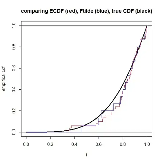
# now lets look at what a single realization might look like
dat <- draw(n)
plot(NA, xlim=0:1, ylim=0:1, xlab="t", ylab="empirical cdf",
     main="comparing ECDF (red), Ftilde (blue), true CDF (black)")
s <- seq(0,1,length=1000)
lines(s, pD(s), lwd=3) # truth in black
abline(h=0:1)
lines(c(0,rep(dat$x,each=2),Inf),
     rep(seq(0,1,length=n+1),each=2),
     col="red")
lines(c(0,rep(which(dat$y==1)/n, each=2),1),
      rep(seq(0,1,length=dat$z+1),each=2),
      col="blue")

EDITS:

EDIT 1 --

I edited this to address @whuber's comments.

EDIT 2 --

I added R code and cleaned it up a bit more. I changed notation slightly for readability, but it is essentially the same. I'm planning on putting a bounty on this as soon as I'm allowed to, so please let me know if you want further clarifications.

EDIT 3 --

I think I addressed @cardinal's remarks. I fixed the typos in the total variation. I'm adding a bounty.

EDIT 4 --

Added a "motivation" section for @cardinal.

Answer 1

While this reference

EDIT: ADDED REFERENCE TO VERY SIMILAR STATISTIC "Nonparametric Estimation from Incomplete Observations" E. L. Kaplan and Paul Meier, Journal of the American Statistical Association, Vol. 53, No. 282 (Jun., 1958), pp. 457-481

is not to your ECDF-like estimator on $[0,1]$ I believe it is logically equivalent to the Kaplan-Meier estimator (aka. product limit estimator) as used in Survival Analysis, even though that's applied to a time range $[0,\infty)$.

Estimating the bias would be possible once you have a reasonable estimate of the distribution via kernel smoothing if it is well enough behaved (see, e.g., Khmaladze transformation on Wikipedia).

In the bivariate case in your graph problem estimating $f = W / \iint W$ from $A$ albeit with a trivial symmetry constraint seems similar to the approach in Jean-David Fermanian, Dragan Radulovic, and Marten Wegkamp (2004), Weak convergence of empirical copula processes, Bernoulli, vol. 10, no. 5, 847–860, as @cardinal indicated "Multivariate Delta Method".

Answer 2

This answers questions 2 and 3 above. I still really want a reference though (from question 1).

This doesn't yet take into account when $\sum Y_i = 0$.

Consider $g(A,B) = A/(A+B)$, then \begin{align} g_A(A,B) &= (A+B)^{-1} + A(A+B)^{-2}\\ g_B(A,B) &= -A(A+B)^{-2}\\ g_{AA}(A,B) &= 2B(A+B)^{-3}\\ g_{AB}(A,B) &= (A-B)(A+B)^{-3}\\ g_{BB}(B,B) &= 2A(A+B)^{-3} \end{align} where the subscripts denote the derivatives. Recall $p_i = f((i-1+U_i)/n)/c$. Let \begin{align} R = \frac{1}{n}\sum_{i=1}^{\lceil nt \rceil} Y_i, \quad& \mu_R = \mathbb{E}(R) = \int_0^t p(u) \, d u = c^{-1}F(t)\\ S = \frac{1}{n}\sum_{\lceil nt \rceil +1}^n Y_i, \quad& \mu_S = \mathbb{E}(S) = \int_t^1 p(u) \, d u = c^{-1}(1-F(t)) \end{align} So note that $\mu_R + \mu_S = c^{-1}F(t) + c^{-1}(1-F(t)) = c^{-1}$ and $g(\mu_R, \mu_S) = F(t)$. Also, \begin{align} \text{ Var}(R) &= \frac{1}{n^2} \sum_{i=1}^{\lceil nt \rceil} \text{ Var}(Y_i) = \frac{1}{n} \int_0^t f(u)/c(1-f(u)/c) \, d u = \frac{1}{nc^2} \int_0^t f(u)(c-f(u)) \, d u\\ \text{ Var}(S) &= \frac{1}{nc^2} \int_t^1 f(u)(c-f(u)) \, d u \end{align} Note that $\text{ Cov}(R,S) = 0$ by independence of the $Y_i$s.

Now, we use a taylor expansion to get \begin{align} &\mathbb{E}\left(\tilde{F}_n(t)\right) =\mathbb{E}\left( \frac{1}{\sum_{i=1}^n Y_i} \sum_{i=1}^{\lceil tn \rceil} Y_i \right) =\mathbb{E}\left(\frac{nR}{nR+nS}\right) =\mathbb{E}\left(\frac{R}{R+S}\right) =\mathbb{E}\left(g(R,S)\right)\\ &=g(\mu_R,\mu_S) + \frac{1}{2}\mathbb{E}((R - \mu_R)^2)g_{RR}(\mu_R, \mu_S) \nonumber\\ &\quad + \mathbb{E}((R - \mu_R)(S-\mu_S))g_{RS}(\mu_R, \mu_S) + \frac{1}{2}\mathbb{E}((S - \mu_S)^2)g_{SS}(\mu_R, \mu_S) + \dots \\ &= F(t) + \frac{1}{2}\mathbb{E}((R - \mu_R)^2)2\mu_S(\mu_R+\mu_S)^{-3} \nonumber\\ &\quad + \mathbb{E}((R - \mu_R)(S-\mu_S))(\mu_R-\mu_S)(\mu_R+\mu_S)^{-3} \nonumber\\ &\quad + \frac{1}{2}\mathbb{E}((S - \mu_S)^2) 2\mu_R(\mu_R+\mu_S)^{-3} + \dots\\ &= F(t) + (\mu_R+\mu_S)^{-3} \bigg( \mathbb{E}((R - \mu_R)^2)\mu_S + \mathbb{E}((R - \mu_R)(S-\mu_S))(\mu_R-\mu_S) \nonumber\\ &\quad + \mathbb{E}((S - \mu_S)^2) \mu_R \bigg) + \dots \\ &= F(t) + c^3 \left( \text{ Var}(R)c(1-F(t)) \right. \nonumber\\ &\quad + \left.\text{ Cov}(R,S)(cF(t) - c(1-F(t))) + \text{ Var}(S) cF(t) \right) + \dots \\ &= F(t) + c^4 \left( \left(\frac{1}{n} \int_0^t f(u)(c-f(u)) \, d u\right) (1-F(t)) \right. \nonumber\\ &\quad \left. + \left(\frac{1}{n} \int_t^1 f(u)(c-f(u)) \, d u \right) F(t) \right) + \dots\\ &= F(t) + \tilde{V}_{F(t)}/n + \dots\\ &= F(t) + {\cal O}(n^{-1}) \end{align} where \begin{align} \tilde{V}_{F(t)} &= c^2\left(\int_0^t f(u)(c-f(u)) \, d u\right) (1-F(t)) + c^2\left(\int_t^1 f(u)(c-f(u)) \, d u \right) F(t)\\ &< c^2\left( \int_0^t cf(u) \, d u\right)(1 - F(t)) + c^2\left( \int_t^1 cf(u) \, d u\right)F(t)\\ &< c^3 2F(t)(1-F(t)) \end{align} In particular, we get \begin{align} \sqrt{n}\left(\tilde{F}_n(t) - F(t)\right) \overset{d}{\to} N(0,V_{F(t)}) \end{align}

Please comment if you see something wrong with this.

EDITS:

Edit 1 --

Fixed a typo in $V_{F(t)}$. Thanks @cardinal for your suggestion in the comments about question 4.

Edit 2 --

Fixed plenty of typos: I had $c^{-1}$ where I should have had $c$ in many places. I still need to address @cardinal's response about $\sum Y_i = 0$.