12

For analyzing data from a biophysics experiment, I'm currently trying to do curve fitting with a highly non-linear model. The model function looks basically like:

$y = ax + bx^{-1/2}$

Here, especially the value of $b$ is of great interest.

A plot for this function:

Function plot

(Note that the model function is based on a thorough mathematical description of the system, and seems to work very well --- it's just that automated fits are tricky).

Of course, the model function is problematic: fitting strategies I've tried thus far, fail because of the sharp asymptote at $x=0$, especially with noisy data.

My understanding of the issue here is that simple least-squares fitting (I've played with both linear and non-linear regression in MATLAB; mostly Levenberg-Marquardt) is very sensitive to the vertical asymptote, because small errors in x are hugely amplified.

Could anyone point me to a fitting strategy that could work around this?

I have some basic knowledge of statistics, but that's still pretty limited. I'd be eager to learn, if only I'd know where to start looking :)

Thanks a lot for your advice!

Edit Begging your pardon for forgetting to mention the errors. The only significant noise is in $x$, and it's additive.

Edit 2 Some additional information about the background of this question. The graph above models the stretching behavior of a polymer. As @whuber pointed out in the comments, you need $b \approx -200 a$ to get a graph like above.

As to how people have been fitting this curve up to this point: it seems that people generally cut off the vertical asymptote until they find a good fit. The cutoff choice is still arbitrary, though, making the fitting procedure unreliable and unreproducible.

Edit 3&4 Fixed graph.

Glen_b
  • 257,508
  • 32
  • 553
  • 939
onnodb
  • 223
  • 2
  • 8
  • 3
    Do the errors come in $x$ or in $y$ or both? In what form do you expect noise to enter (multiplicative, additive, etc.)? – probabilityislogic Mar 13 '13 at 12:09
  • @probabilityislogic Thanks for pointing that out! Question edited. – onnodb Mar 13 '13 at 18:11
  • When you say fitting strategies fail, what exactly happens? – curious_cat Mar 13 '13 at 18:20
  • @curious_cat They produce fits that are clearly off (visually). If I simulate data, and fit them again, I get wildly different parameter values, combined with fits that *look* bad. Cutting off the vertical asymptote helps, but then the fit parameters tend to depend on the cutoff position. Does that answer your question? Thanks for chiming in! – onnodb Mar 13 '13 at 18:25
  • 2
    @onnodb: My concern is, might this not fundamentally question how robust your model itself is? No matter what fitting strategy you use won't $b$ remain highly sensitive? Can you ever have a high confidence in such an estimate for $b$? – curious_cat Mar 13 '13 at 18:34
  • @onnodb: Also, how many data points do you have? And how many fall in that initial spike region? – curious_cat Mar 13 '13 at 18:36
  • @curious_cat The robustness question is a very good one, and one I've been worrying about a lot. Still, I do feel that producing a good fit *should* be possible, since doing it by hand seems easy enough. Would there be a way to have a least-squares error based on 'proximity' in the x-y plane, instead of x or y error? (Or is that a silly question?) Regarding the number of data points: this can be arbitrarily high (thousands of points would be no problem). Since in the experiment we actually control $y$, especially the vertical asymptote is easy to measure very fine-grained. – onnodb Mar 13 '13 at 18:42
  • @onnodb: About your proximity question: "PCA effectively minimizes error orthogonal to the model" Look here: http://i.stack.imgur.com/bOl5N.png and http://stats.stackexchange.com/questions/2691/making-sense-of-principal-component-analysis-eigenvectors-eigenvalues Though, I'm not sure if or not this is relevant. – curious_cat Mar 13 '13 at 19:17
  • Hm, yeah, but PCA would only be useful for fitting a linear model --- unless you start looking into nonlinear PCA algorithms, but I don't think they'd be useful. Thanks for the suggestion, though! – onnodb Mar 13 '13 at 19:20
  • I cannot make a graph of $y = a x + b / \sqrt{x}$ look like the one shown here until I introduce a sizable additive constant. What exactly is this figure depicting? – whuber Mar 13 '13 at 22:58
  • @whuber Good point; see Edit 2. – onnodb Mar 14 '13 at 07:48
  • 1
    Unfortunately, that still won't work. There simply is no possible combination of $a$ and $b$ that will even qualitatively reproduce the graph you have drawn. (Obviously $b$ is negative. $a$ must be less than the least slope in the graph, yet positive, which puts it into a narrow interval. But when $a$ is in that interval, it simply is not large enough to overcome the huge negative spike at the origin introduced by the $b x^{1/2}$ term.) What have you drawn? Data? Some other function? – whuber Mar 14 '13 at 07:58
  • @whuber Apologies, the bit to the right was indeed incorrect --- a leftover from a different model function which is besides the point. The current graph should be fine. – onnodb Mar 15 '13 at 09:30
  • 1
    Thanks, but it's still wrong. Extending the tangent to this graph backwards from *any* point $(x,ax+bx^{1/2})$ where $x\gt 0$, you will intercept the y-axis at $(0,3b/(2x^{1/2}))$. Because the downward spike at $0$ shows $b$ is negative, this y-intercept has to be negative, too. But in your figure it is abundantly clear that most such intercepts are positive, extending as high as $15.5$. Thus **it is mathematically impossible that an equation like $y=ax + bx^{1/2}$ can describe your curve**, *not even approximately.* At a minimum you need to fit something like $y=ax+bx^{1/2}+c$. – whuber Mar 15 '13 at 15:20
  • @whuber Of course, you are absolutely right. Pardon my sloppiness --- experimental physicist at work ;) Graph is fixed now. Basic problem is still the same though: how to fit a function that displays asymptotic behavior in both the $x$ and $y$ direction? Discussion with other people suggest that very high-precision data would be needed for the vertical asymptote regime, and then it might work without problems. – onnodb Mar 15 '13 at 20:52
  • 1
    Before I did any work on this, I wanted to make sure of the statement of the question: that's why it's important to get the function correct. I haven't time to give a full answer now, but would like to remark that "other people" may be wrong--but it depends on yet more details, alas. If your $x$ error is truly *additive* it seems to me it must still be strongly heteroscedastic, for otherwise its variance at small values of $x$ would be truly tiny. What can you tell us--quantitatively--about that error? – whuber Mar 15 '13 at 21:52
  • Yes, thanks for correcting the graph, @whuber. Of course, I'm happy to provide more details! $x$ is the force on a polymer, which we can measure with a precision of around 0.5--1 (bottleneck being instrument noise). Variance in $x$ stays the same over the whole range of $y$, basically. Does that help? – onnodb Mar 16 '13 at 07:58

3 Answers3

10

The methods we would use to fit this manually (that is, of Exploratory Data Analysis) can work remarkably well with such data.

I wish to reparameterize the model slightly in order to make its parameters positive:

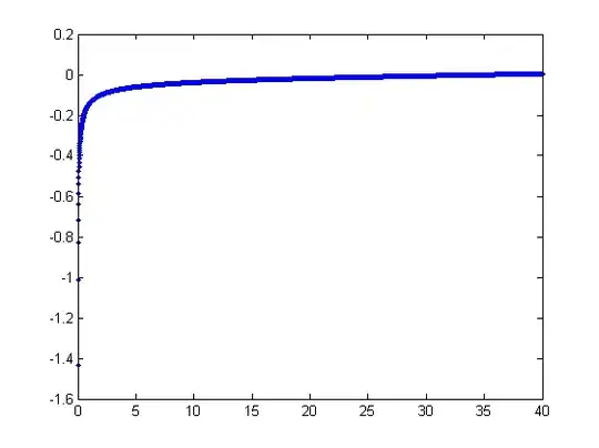
$$y = a x - b / \sqrt{x}.$$

For a given $y$, let's assume there is a unique real $x$ satisfying this equation; call this $f(y; a,b)$ or, for brevity, $f(y)$ when $(a,b)$ are understood.

We observe a collection of ordered pairs $(x_i, y_i)$ where the $x_i$ deviate from $f(y_i; a,b)$ by independent random variates with zero means. In this discussion I will assume they all have a common variance, but an extension of these results (using weighted least squares) is possible, obvious, and easy to implement. Here is a simulated example of such a collection of $100$ values, with $a=0.0001$, $b=0.1$, and a common variance of $\sigma^2=4$.

Data plot

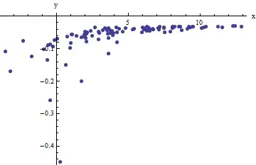
This is a (deliberately) tough example, as can be appreciated by the nonphysical (negative) $x$ values and their extraordinary spread (which is typically $\pm 2$ horizontal units, but can range up to $5$ or $6$ on the $x$ axis). If we can obtain a reasonable fit to these data that comes anywhere close to estimating the $a$, $b$, and $\sigma^2$ used, we will have done well indeed.

An exploratory fitting is iterative. Each stage consists of two steps: estimate $a$ (based on the data and previous estimates $\hat{a}$ and $\hat{b}$ of $a$ and $b$, from which previous predicted values $\hat{x}_i$ can be obtained for the $x_i$) and then estimate $b$. Because the errors are in x, the fits estimate the $x_i$ from the $(y_i)$, rather than the other way around. To first order in the errors in $x$, when $x$ is sufficiently large,

$$x_i \approx \frac{1}{a}\left(y_i + \frac{\hat{b}}{\sqrt{\hat{x}_i}}\right).$$

Therefore, we may update $\hat{a}$ by fitting this model with least squares (notice it has only one parameter--a slope, $a$--and no intercept) and taking the reciprocal of the coefficient as the updated estimate of $a$.

Next, when $x$ is sufficiently small, the inverse quadratic term dominates and we find (again to first order in the errors) that

$$x_i \approx b^2\frac{1 - 2 \hat{a} \hat{b} \hat{x}^{3/2}}{y_i^2}.$$

Once again using least squares (with just a slope term $b$) we obtain an updated estimate $\hat{b}$ via the square root of the fitted slope.

To see why this works, a crude exploratory approximation to this fit can be obtained by plotting $x_i$ against $1/y_i^2$ for the smaller $x_i$. Better yet, because the $x_i$ are measured with error and the $y_i$ change monotonically with the $x_i$, we should focus on the data with the larger values of $1/y_i^2$. Here is an example from our simulated dataset showing the largest half of the $y_i$ in red, the smallest half in blue, and a line through the origin fit to the red points.

Figure

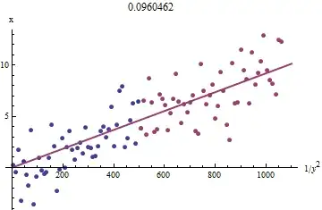
The points approximately line up, although there is a bit of curvature at the small values of $x$ and $y$. (Notice the choice of axes: because $x$ is the measurement, it is conventional to plot it on the vertical axis.) By focusing the fit on the red points, where curvature should be minimal, we ought to obtain a reasonable estimate of $b$. The value of $0.096$ shown in the title is the square root of the slope of this line: it's only $4$% less than the true value!

At this point the predicted values can be updated via

$$\hat{x}_i = f(y_i; \hat{a}, \hat{b}).$$

Iterate until either the estimates stabilize (which is not guaranteed) or they cycle through small ranges of values (which still cannot be guaranteed).

It turns out that $a$ is difficult to estimate unless we have a good set of very large values of $x$, but that $b$--which determines the vertical asymptote in the original plot (in the question) and is the focus of the question--can be pinned down quite accurately, provided there are some data within the vertical asymptote. In our running example, the iterations do converge to $\hat{a} = 0.000196$ (which is almost twice the correct value of $0.0001$) and $\hat{b} = 0.1073$ (which is close to the correct value of $0.1$). This plot shows the data once more, upon which are superimposed (a) the true curve in gray (dashed) and (b) the estimated curve in red (solid):

Fits

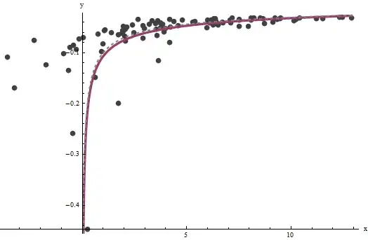
This fit is so good that it is difficult to distinguish the true curve from the fitted curve: they overlap almost everywhere. Incidentally, the estimated error variance of $3.73$ is very close to the true value of $4$.

There are some issues with this approach:

  • The estimates are biased. The bias becomes apparent when the dataset is small and relatively few values are close to the x-axis. The fit is systematically a little low.

  • The estimation procedure requires a method to tell "large" from "small" values of the $y_i$. I could propose exploratory ways to identify optimal definitions, but as a practical matter you can leave these as "tuning" constants and alter them to check the sensitivity of the results. I have set them arbitrarily by dividing the data into three equal groups according to the value of $y_i$ and using the two outer groups.

  • The procedure will not work for all possible combinations of $a$ and $b$ or all possible ranges of data. However, it ought to work well whenever enough of the curve is represented in the dataset to reflect both asymptotes: the vertical one at one end and the slanted one at the other end.


Code

The following is written in Mathematica.

estimate[{a_, b_, xHat_}, {x_, y_}] := 
  Module[{n = Length[x], k0, k1, yLarge, xLarge, xHatLarge, ySmall, 
    xSmall, xHatSmall, a1, b1, xHat1, u, fr},
   fr[y_, {a_, b_}] := Root[-b^2 + y^2 #1 - 2 a y #1^2 + a^2 #1^3 &, 1];
   k0 = Floor[1 n/3]; k1 = Ceiling[2 n/3];(* The tuning constants *)
   yLarge = y[[k1 + 1 ;;]]; xLarge = x[[k1 + 1 ;;]]; xHatLarge = xHat[[k1 + 1 ;;]];
   ySmall = y[[;; k0]]; xSmall = x[[;; k0]]; xHatSmall = xHat[[;; k0]];
   a1 = 1/
     Last[LinearModelFit[{yLarge + b/Sqrt[xHatLarge], 
          xLarge}\[Transpose], u, u]["BestFitParameters"]];
   b1 = Sqrt[
     Last[LinearModelFit[{(1 - 2 a1 b  xHatSmall^(3/2)) / ySmall^2, 
          xSmall}\[Transpose], u, u]["BestFitParameters"]]];
   xHat1 = fr[#, {a1, b1}] & /@ y;
   {a1, b1, xHat1}
   ];

Apply this to data (given by parallel vectors x and y formed into a two-column matrix data = {x,y}) until convergence, starting with estimates of $a=b=0$:

{a, b, xHat} = NestWhile[estimate[##, data] &, {0, 0, data[[1]]}, 
                Norm[Most[#1] - Most[#2]] >= 0.001 &,  2, 100]
whuber
  • 281,159
  • 54
  • 637
  • 1,101
  • 3
    This is an amazing answer; I'm much obliged! I've been playing with this, and the results look very promising. I'll need a bit more time to fully understand the reasoning, though :) Also: could I contact you through your website for one additional (private) question, regarding acknowledgements? – onnodb Mar 19 '13 at 10:48
3

See the important questions @probabilityislogic posted

If you only have errors in y, and they're additive and you have constant variance (i.e. your assumptions fit what it sounds like you did), then if you let $y^* = y\sqrt{x}$, you could perhaps try a weighted linear fit of $y^*$ on $x^* = x^{3/2}$, where the weights will then be proportional to $1/x$ ... (and yes, this might simply be shifting the problem around, so it may still be problematic - but you should at least find it easier to regularize with this transformation of the problem).

Note that with this manipulation, your $b$ becomes the intercept of the new equation

If your variances are already not constant or your errors aren't additive or you have errors in the $x$, this will change things.

--

Edit to consider the additional information:

We got to a model of the form: $y^* = b + a x^*$

We now have that the errors are in x and additive. We still don't know if the variance is constant on that scale.

Rewrite as $x^* = y^*/a - b/a = m y^* + c$

Let $x_o^* = x^* + \eta$, where this error term may be heteroskedastic (if the original $x$ has constant spread, it will be heteroskedastic, but of known form)

(where the $o$ in $x_o^*$ stands for 'observed')

Then $x^*_o = c + m y^* + \epsilon$ where $\epsilon = -\zeta$ looks nice but now has correlated errors in the $x$ and $y$ variables; so it's a linear errors-in-variables model, with heteroskedasticity and known form of dependence in the errors.

I am not sure that improves things! I believe there are methods for that kind of thing, but it's not really my area at all.

I mentioned in the comments that you might like to look at inverse regression, but the particular form of your function may preclude getting far with that.

You might even be stuck with trying fairly robust-to-errors-in-x methods in that linear form.

--

Now a huge question: if the errors are in x, how the heck were you fitting the nonlinear model? Were you just blindly minimizing the sum of squared errors in $y$? That might well be your problem.

I suppose one could try to rewrite the original thing as a model with errors in the $x$ and try to optimize the fit but I am not sure I see how to set that up right.

Glen_b
  • 257,508
  • 32
  • 553
  • 939
  • Thanks! It's an interesting transformation, hadn't thought of that --- even though the errors are in $x$, I'll play around with it anyway! – onnodb Mar 13 '13 at 18:18
  • 2
    "*even though the errors are in x*" -- yikes, that's kind of important. You may want to check up on inverse regression. – Glen_b Mar 13 '13 at 21:34
  • 3
    ...or you could directly fit the model $x = \frac{1}{3} \left(\frac{2 y}{a}+\frac{2^{1/3} y^2}{\left(27 a^4 b^2-2 a^3 y^3+3 \sqrt{3} \sqrt{27 a^8 b^4-4 a^7 b^2 y^3}\right)^{1/3}}+\frac{\left(27 a^4 b^2-2 a^3 y^3+3 \sqrt{3} \sqrt{27 a^8 b^4-4 a^7 b^2 y^3}\right)^{1/3}}{2^{1/3} a^2}\right)$ :-). – whuber Mar 13 '13 at 21:58
  • @whuber Hmm. Solving for the cubic, clever. If we write the original in terms of $x_o$ where $x_o$ is $x + \zeta$, this would leave us with $x = (\rm{that\,\, monster}) + \epsilon\,$, (again with $\epsilon = -\zeta$) which at least notionally can be done with nonlinear least squares. So that looks like it takes care of the error propagation properly. It *might* actually work if the OP was to use the linear form I was playing with (using some robust-to-errors-in-the-IV-and-hetero estimation) to get good starting values for the parameters and then try to use this nonlinear LS form to polish it. – Glen_b Mar 13 '13 at 22:18
  • I believe linearizing the function $x(y)$ and (ironically) applying nonlinear (weighted) least squares would work, especially if the data were restricted to relatively small values of $y$ where the curve is primarily determined by $b$. – whuber Mar 13 '13 at 22:42
  • Thanks for the extensive reply, Glen. I'll have to sit down and study this, which might take a few days (I'm leaving for a short conference this morning). I'll get back to you, though! Thanks again! – onnodb Mar 14 '13 at 07:49
0

After some more weeks of experimenting, a different technique seems to work the best in this particular case: Total Least Squares fitting. It's a variant of the usual (nonlinear) Least Squares fitting, but instead of measuring fit errors along just one of the axes (which causes problems in highly nonlinear cases such as this one), it takes both axes into account.

There's a plethora of articles, tutorials and books avaiable on the subject, although the nonlinear case is more elusive. There's even some MATLAB code available.

onnodb
  • 223
  • 2
  • 8
  • Thanks for sharing this. I accept that it it might produce good-looking results in your case, but I have two concerns. The first you mention: how exactly does one apply total least squares/errors-in-variables regression/orthogonal regression/Deming regression to nonlinear fits? The second is that this approach does not seem appropriate for your data, in which $y$ is measured essentially without error. When that's the case, you should *not* be allowing for residuals in the $y$ variable and doing so *ought* to produce unreliable, biased results. – whuber Apr 16 '13 at 15:49
  • @whuber Thanks for expressing your concerns! Right now, I'm still working on running simulations to probe the reliability of TLS fitting for this problem. What I've seen thus far, though, is that TLS' consideration of *both* variables helps greatly in overcoming the high non-linearity of the model. Fits of simulated data are reliable and converge very well. More work needs to be done though, and I'll definitely have to stack your method up to this one, once we have more actual data available --- and look in detail into your concerns. – onnodb Apr 16 '13 at 19:22
  • OK--don't forget I have comparable concerns about the method I proposed! – whuber Apr 16 '13 at 21:07