Can a random variable be uncorrelated with its product with a correlated random variable?

Question

I have a random variable $X.$ I want to find a random variable $Y$ such that $Y$ is correlated with $X,$ but $Y$ is not correlated with the product of $X$ and $Y.$ Is it always possible?

Answer 1

If $X=Y$ and Rademacher distributed, the product will be a constant and have zero covariance (uncorrelated) with $X$ or $Y$.

Is it always possible?

My previous example was incorrect.

Answer 2

Provided $X$ is non-degenerate (that is, it is not almost surely constant) and has finite variance (without which it's impossible to have any correlation), you can always find such a $Y.$

One method begins by taking any random variable $Y_0$ for which $E[Y_0]=0$ but $E[XY_0]\ne 0$ and $E[|X|\,Y_0^2] \lt \infty.$ There always exists such a variable when $X$ is non-constant. Rather than go into this technical detail, let's limit the analysis to random variables $X$ for which $E[|X|^3]$ is finite, where it's simple to construct a variable with these properties: just set $Y_0 = X-E[X].$ This guarantees $E[Y_0]=0.$ Calculate

$$E[XY_0] = E[X(X-E[X])] = E[X^2] - E[X]^2 = \operatorname{Var}(X)\ne 0$$

because $X$ is non-constant. Finally,

$$E[|X|\,Y_0^2] = E[|X|^3] - 2E[X]E[X\,|X|] + E[X]^2E[|X|] \lt \infty$$

is guaranteed by the power norm inequality.

Define

$$\eta = -\frac{E[XY_0^2]}{E[XY_0]}.$$

This number always exists because the denominator is nonzero, and the numerator is finite. Set

$$Y = Y_0 + \eta$$

and compute

$$\begin{aligned} E[Y] &= \eta\\ E[XY] &= E[XY_0] + \eta E[X]\\ E[XY^2] &= E[XY_0^2] + 2\eta E[XY_0] + \eta^2E[X]. \end{aligned}$$

Use these to find

$$\begin{aligned} \operatorname{Cov}(X,Y) &= E[XY] - E[X]E[Y] = E[XY_0]\ne 0 \text{ and}\\ \operatorname{Cov}(XY,Y) &= E[XY_0^2] + \eta E[XY_0] = 0 \end{aligned}$$

(due to the definition of $\eta:$ now you see where it came from!). The correlations are just scaled versions of these covariances, whence the correlation of $X$ and $Y$ is nonzero but the correlation of $XY$ and $Y$ is zero.

---

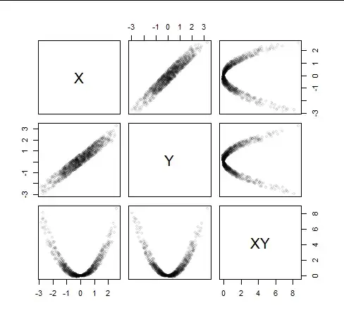
In practice it helps to add a tiny amount of noise to $Y_0:$ this will deal with the more difficult situations such as when $X$ has only two values and one of them is rare. As an example, I have added a little bit of uniform noise to a Normally generated $X$ and carried out the preceding construction (viewing the values as an empirical probability distribution). Here are the scatterplots:

It is clear what's going on: Because $Y$ parallels $X,$ $X$ and $Y$ are (strongly positively) correlated, as shown in the middle top and middle left panels. But because $Y$ has been suitably centered (that's the role of $\eta$), the relation between $Y$ and $XY$ is parabolic, with arms just balancing one another out to assure zero correlation: that is what the middle bottom and middle right panels show. (The other two panels in the upper right and lower left corners are irrelevant.)

This is the R code that generated the figure.

#
# Generate a random variable.
# (This is an empirical distribution).
#
# x <- rbinom(1e4, 1, 9/10) # A difficult test
x <- rnorm(1e3)
#
# Find Y.
#
eps <- diff(range(x)) * 1e-1
y <- x + runif(length(x), -eps, eps)
y <- y - mean(y)
eta <- -mean(x*y^2) / mean(x*y)
y <- y + eta
#
# Exhibit the correlation coefficients as a check.
#
zapsmall(c(`rho(x,y)`=cor(x,y), `rho(xy,y)`=cor(x*y, y)))
#
# Display the scatterplots.
#
pairs(cbind(X=x, Y=y, XY=x*y), pch=19, cex=.8, col="#00000010")