If you know the sample size (as opposed to just knowing that the sample size is between 50 and 200), then maximum likelihood might work in this case. Using Mathematica:
(* Joint distribution of largest 4 order statistics from a sample size of 100 *)
dist = OrderDistribution[{NormalDistribution[0, \[Sigma]], 100}, {97, 98, 99, 100}];

(* Log of the likelihood *)
logL = Log[PDF[dist, {x97, x98, x99, x100}][[1, 1, 1]]];
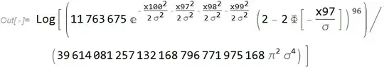
This can be simplified a bit and upon removing additive constants we have
$$96\log \left(\Phi \left(\frac{x_{97}}{\sigma }\right)\right)-4 \log (\sigma )-\frac{x_{97}^2+x_{98}^2+x_{99}^2+x_{100}^2}{2 \sigma ^2}$$
where $\Phi(.)$ is the unit normal cdf. We just find the value of $\sigma$ that maximizes the above equation. In general if you just have the largest $k$ observations labeled $x_{n-k+1},x_{n-k},\ldots,x_n$ for a sample size of $n$, then the log of the likelihood is (excluding the additive constants):
$$(n-k)\log\left(\Phi\left(x_{n-k+1}/\sigma\right)\right)-k\log(\sigma)-{{1}\over{2\sigma^2}}\sum_{i=n-k+1}^n x_i^2$$
Note that this is highly dependent on being able to assume (as opposed to just being willing to assume) that the samples are all independent and from the same normal distribution with mean 0. It's not often that happens.
(* Generate some data *)
SeedRandom[12345];
x = Sort[RandomVariate[NormalDistribution[0, 1], 100]];
data = {x97 -> x[[97]], x98 -> x[[98]], x99 -> x[[99]], x100 -> x[[100]]};

(* Obtain maximum likelihood estimate of \[Sigma] *)
mle = FindMaximum[{logL /. data, \[Sigma] > 0}, {{\[Mu], 0}, {\[Sigma], 1}}]
(* {2.00775, {\[Sigma] -> 0.931452}} *)

(* Estimated variance and standard error of the estimator of \[Sigma] *)
var\[Sigma] = -1/(D[logL /. data, {\[Sigma], 2}]) /. mle[[2]]
se\[Sigma] = var\[Sigma]^0.5
(* 0.110698 *)
Addition
If there are $s$ independent sets of samples of size $n_i$ where only the last $k_i$ observations are available (with $i=1,2,\ldots,s$), then one can sum the individual log likelihoods and maximize that function to get the maximum likelihood estimate:
$$\log{L}=-\frac{\sum _{i=1}^s \sum _{j=-k_i+n_i+1}^{n_i} x_{i,j}}{2 \sigma ^2}+\sum _{i=1}^s (n_i-k_i) \log \left(\Phi \left(\frac{x_{i,n_i-k_i+1}}{\sigma }\right)\right)-\log (\sigma ) \sum _{i=1}^s k_i$$
Then take the reciprocal of minus the second derivative of $\log{L}$ with respect to $\sigma$ and plug in $\hat{\sigma}$ for $\sigma$ to get an estimate of the variance.
While a symbolic representation of the estimated variance can be obtained, in practice that is probably not very useful. Whatever optimization routine is used will likely produce something that will get you what you need. Consider the single set of observations and the use of R:
# Generate some data
  n <- 100  # Sample size
  sigma <- 1
  set.seed(12345)
  x <- sigma*rnorm(n) # Normal with mean zero and sd sigma
# Now keep just the highest 4 values
  x <- x[order(x)][(n-3):n]

# Define log likelihood function
  logL <- function(sigma, n, x) {
    k <- length(x)
    (n-k)*log(pnorm(x[1]/sigma)) - k*log(sigma) - sum((x/sigma)^2)/2
  }

# Find maximum likelihood estimate of sigma
# Using mean(x)/2 is a reasonable starting value when n=100
  result <- optim(mean(x)/2, logL, n=n, x=x, method="L-BFGS-B",
    lower=0, upper=Inf, control=list(fnscale=-1), hessian=TRUE)
  result$par
  # 1.111482

# Now estimate the standard error
  se <- (-solve(result$hessian))^0.5
  se
  # 0.1376703
For multiple sets of data it depends on how you set up the data structure. In the example below I put the information for each set of data in a separate list element.
# Generate some data
  nSets = 4 # Number of data sets
  n <- pmax(100,rpois(nSets, 150))  # Sample size
  k <- pmax(2, rpois(nSets, 5))     # Largest k observations available
  sigma <- 1
  set.seed(12345)
  y <- vector(mode = "list", length = nSets)  # Empty list
  for (i in 1:nSets) {
      y[[i]]$n <- n[i]
      x = sigma*rnorm(n[i]) # Normal with mean zero and sd sigma

      # Now keep just the highest k[i] values
      x <- x[order(x)][(n[i]-k[i]+1):n[i]]
      y[[i]]$x <- x
  }

# Define log likelihood function
  logL <- function(sigma, n, x) {
    k <- length(x)
    (n-k)*log(pnorm(x[1]/sigma)) - k*log(sigma) - sum((x/sigma)^2)/2
  }

# Define sum of log likelihood functions
  sumlogL <- function(sigma, y) {
    s = 0
    for (i in 1:length(y)) {
        s = s + logL(sigma, y[[i]]$n, y[[i]]$x)
    }
    s
  }

# Find maximum likelihood estimate of sigma
  result <- optim(mean(y[[1]]$x)/2, sumlogL, y=y, method="L-BFGS-B",
    lower=0, upper=Inf, control=list(fnscale=-1), hessian=TRUE)
  result$par
  # 1.058365

# Now estimate the standard error
  se <- (-solve(result$hessian))^0.5
  se
  # 0.05002775
Alternatively if the $k_i$ are all equal and the $n_i$ are close to being equal, then just take the mean of the individual estimates and use the usual formula for a sample standard deviation to obtain an estimate of $\sigma$.

