About piecewise linear functions
You are given two piecewise linear functions. A function $f$ is piecewise linear when it is "locally linear." That is, for every $x$ in its domain there is an interval $I\ni x$ and constants $\alpha_I,$ $\beta_I$ for which
$$f_{\mid I}(x) = \alpha_I + \beta_I x.$$
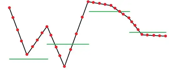
Your representation of these functions appears to be in terms of their graphs, which are unions of line segments that, if they intersect at all, intersect only at endpoints. For instance, the function $f$ with the black graph is the union of eight such segments connecting the nine red endpoints. The function $g$ with the green graph also is the union of four segments. (Notice that a piecewise linear function needn't be continuous!) Let's call the $x$ values of the segments defining $f$ its "breaks."
The union of the breaks for $f$ and the breaks for $g$ determines the only points at which $f$ or $g$ may have "kinks" or "breaks." As a first step, we may insert points into their graphs (wherever needed) so that $f$ and $g$ share the same set of breaks. If $f$ and $g$ are not defined on the same domain, at this juncture we will also want to restrict them to the intersection of their domains, for otherwise it will make no sense to subtract them and carry out further calculations of that sort.
This figure shows functions like those in the question. (I have modified them slightly in order to illustrate what happens when $f$ (black graph) and $g$ (green graph) do not originally have the same breaks.) The values of these functions at their breaks are highlighted (as in the question) with point symbols.

The tan graph plots the difference $h = f-g.$ Notice that its breaks are the union of the breaks of $f$ and $g.$
Integrating piecewise linear functions
We have achieved a representation of $h$ as a collection of linear functions defined on a set of intervals. This makes it easy to integrate its square:
$$\begin{aligned}
\int h^2(x)\,\mathrm{d}x
&= \sum_I \int_I h_{\mid I}^2(x)\,\mathrm{d}x \\
&= \sum_I \int_I (\alpha_I + \beta_I x)^2\,\mathrm{d}x \\
&= \sum_I \left(\alpha_I^2 x + \alpha_I\beta_I x^2 + \frac{1}{3}\beta_I^2 x^3\right)\mid_I
\end{aligned}\tag{*}$$
where, as usual, expressions of the form "$u(x)\mid_I$" mean to evaluate $u$ at the endpoints of $I$ and subtract. Thus,
The integral of $h^2 = (f-g)^2$ can be computed with $O(n)$ effort where $n$ is the total number of breakpoints occurring in $f$ and $g.$
The "mean squared error" is just this integral divided by the total lengths of the intervals involved. Take the square root of that to obtain the root mean squared error.
Here is an example of the graph of $h^2$ from the previous figure. Its mean value (that is, the mean squared difference between the original $f$ and $g$) is the height splitting the shaded region into two equal areas for the points above the mean and the points below the mean.

The distribution determined by a piecewise linear function
When $X$ is a random variable uniformly distributed on the domain of $h,$ we may conceive of $X$ as being a mixture of uniform distributions on the segments of $h.$ The mixture weights are, of course, just the relative lengths of the segments.
The distribution of $Y = h(X)$ also is a mixture of uniform distributions. That is because on each interval, $Y$ is a linear transformation of $X$ and linear transformations of uniform distributions are uniform distributions. Consequently, we may use techniques for working with mixture distributions to compute with $Y.$ See https://stats.stackexchange.com/a/122816/919 for a code sample to compute a general mixture density (which applies directly to computing the mixture PDF), https://stats.stackexchange.com/a/411671/919 for computing its quantile function, and https://stats.stackexchange.com/a/64058/919 for drawing values randomly from a mixture.
The next figure plots the distribution determined by the preceding $h$ using these techniques.

Comparing the calculations
We now have an abundance of methods available to compute the mean squared error. They include
The direct calculation $(*).$
Black-box numerical integration of $(f-g)^2.$
Using the density $f_{h(X)},$ where the mean squared error is just the second (raw) moment. It can be computed in various ways, such as by black-box numerical integration of $y^2 f_{h(X)}(y)\,\mathrm{d}y.$
When I carried out these calculations for the running example, the output was
   Direct Numerical   Density
5.9961458 5.9961469 5.9961458
You can see differences in the seventh decimal place, well within the error estimated by the black-box integrator (the integrate function in R). Some error in the block-box integrator is to be expected, because its doesn't know that what it is integrating has a piecewise definition, forcing it to estimate where any jumps or spikes might be and creating (smallish) errors where it interpolates across them.
