Estimating individual components of a mixture distribution

Question

I am trying to jointly estimate the components of a mixture distribution.

I have a sampling from a mixture, XY, composed of X and Y with a known mixing parameter m. I also have a separate sampling of just Y. I am trying to estimate the the PDF of X.

Here is a concrete example.

# Generate XY sampling data
m <- 0.2 # Mixing parameter
n <- 1000
k <- rbinom(1, n, prob = m)
xy <- c(rnorm(n-k, 1, 1), rnorm(k, 5, 0.5))

# Estimate XY_pdf
XY_pdf <- density(xy)
plot(XY_pdf)

# Generate independent Y sampling data
y2 <- rnorm(500, mean = 5, sd = 0.5)
Y_pdf <- density(y2, bw = XY_pdf$bw)
lines(Y_pdf$x, Y_pdf$y*m, col = "red", lty=2)

# Function for calculating P_kde; https://stackoverflow.com/a/34682302/2723734
kde_val <- function(x, t, bw){
  sapply(t, function(ti) {
    kernelValues <- rep(0,length(x))
    for(i in 1:length(x)){
      transformed = (ti - x[i]) / bw
      kernelValues[i] <- dnorm(transformed, mean = 0, sd = 1) / bw
    }
    return(sum(kernelValues) / length(x))
  })
}

t <- seq(-3, 9, by = 0.01)
xy_val <- kde_val(xy, t, XY_pdf$bw)
y_val  <- kde_val(y2, t, Y_pdf$bw) * m
x_val_est <- xy_val - y_val
lines(t, x_val_est, col = "blue")

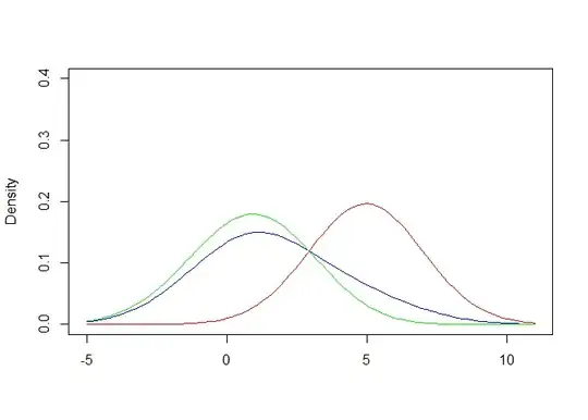
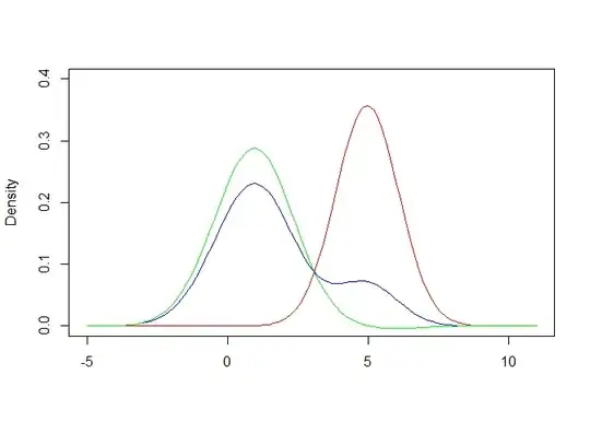
The plot shows PDF(XY) and PDF(Y) estimated from KDE (black and red); and an estimate of PDF(X) = PDF(XY) - PDF(Y)*m (blue).

The estimate of PDF(X) is pretty good, except towards the tail where it becomes negative due to sampling variation in XY and Y.

How do I properly estimate PDF(X)?

(I can't assume the distributions are gaussian)

Answer 1

In the example, you estimated the overall mixture distribution using a KDE, and estimated the second mixture component using a KDE fit to another dataset sampled exclusively from that component. You then tried to obtain the first mixture component by subtracting the latter KDE from the former, scaled by the mixing weight. Unfortunately, this doesn't yield a valid probability density function, as seen by the negative density values in the plot. Furthermore, both datasets contain information about the second mixture component. Estimating this component using only one dataset fails to take advantage of this information, yielding a suboptimal estimate for both mixture components.

A more principled method should simultaneously estimate both mixture components using all available data. Below, I'll describe how to do this using a maximum likelihood approach.

Approach

Changing the notation for clarity, suppose the mixture distribution is:

$$p(x \mid \theta_1, \theta_2) = m p_1(x \mid \theta_1) + (1-m) p_2(x \mid \theta_2)$$

where and $p_1$ and $p_2$ are the mixture components (parameterized by $\theta_1$ and $\theta_2$) and $m \in [0,1]$ is a known parameter controlling the mixing strength. Let $X^A$ be a dataset sampled i.i.d. from the mixture distribution and $X^B$ be a dataset sampled i.i.d. from the second mixture component alone. The log likelihood for both datasets is:

$$L(\theta_1, \theta_2) = \sum_{x \in X^A} \log p(x \mid \theta_1, \theta_2) + \sum_{x \in X^B} \log p_2(x \mid \theta_2)$$

The parameters for both components are simultaneously estimated by maximizing the likelihood for both datasets:

$$\max_{\theta_1, \theta_2} \ L(\theta_1, \theta_2)$$

If a simple parametric form is known for the mixture components, this should be used. Otherwise, the components must be modeled using a flexible family of density functions that can reasonably approximate many possible shapes. For example, each component could itself be represented as a mixture distribution (as in the example below). One could also use spline-based density functions, or various other possibilities.

Example

I generated toy data using $m=0.7$ and Weibull mixture components with different shapes (since the question specifies that they''re non-Gaussian). To mimic the situation where the true parametric family is unknown, I modeled each mixture component as a weighted KDE:

$$p_1(x \mid \theta_1) = \sum_{i=1}^k w^1_i \mathcal{N}(x \mid \mu_i, \sigma^2)$$

$$p_2(x \mid \theta_2) = \sum_{i=1}^k w^2_i \mathcal{N}(x \mid \mu_i, \sigma^2)$$

This approximates each mixture component as a weighted sum of $k$ Gaussian kernels centered over the common 'prototype points' in $\mu$ (which I set equal to $X^A$). Kernels have a fixed bandwidth $\sigma$ (which I set to $0.4$). Unlike a regular KDE, each kernel has a different weight; the two mixture components are distinguished by their different weight vectors $w^1$ and $w^2$. I parameterized the weight vectors using the softmax function. This constrains them to be non-negative and sum to one, ensuring that they're always valid:

$$w^1 = \operatorname{softmax}(\theta_1) \quad w^2 = \operatorname{softmax}(\theta_2)$$

Note that $\theta_1$ and $\theta_2$ are vectors with an entry for each point in $X^A$. I fit them by numerically maximizing the log likelihood $L(\theta_1, \theta_2)$ as described above, using the BFGS algorithm.

The following plot shows the true and estimated mixture distributions, along with the individual mixture components (scaled by $m$ and $1-m$, respectively).

Note that the estimated mixture components are 'leaning in' slightly at the edges. This reflects the difficulty of approximating a skewed, non-Gaussian distribution as a sum of Gaussian kernels with identical bandwidths. This could be resolved by decreasing the kernel bandwidth, allowing the bandwidth to vary across kernels, or by using a different family of approximating distributions. The first two choices would produce a more flexible model, requiring more data.

Answer 2

This is an interesting problem. My basic approach is to fit a kernel density estimate as the question suggested, but adjust the bandwidth to see if I can find a bandwidth for $XY$ and a bandwidth for $Y$ such that $X$ is never negative. I don't think a solution is guaranteed, but it worked in my examples. To find the bandwidths, I used a machine learning approach with a cost function constructed to ensure there are no negative sections of the $X$ pdf and to ensure that the bandwidths don't get inflated. I don't have a reference for this, but I couldn't find anything directly on point here.

Also, note that I think the pdf equation should be: $f_{XY} = (1-m)f_X + mf_Y$ so $f_X = \frac{1}{1-m} (f_{XY} - mf_Y)$

# x = points to evalue density
# xi = data from a random sample of the distribution
# bw = bandwidth
my_density <- function(x, xi, bw)
{
  # kernel is a standard normal pdf
  n <- length(xi)
  return(sapply(x, function(z) {
    1 / n / bw * sum(dnorm((z - xi) / bw))
  }))
};

# par = optimization parameters, bandwidth for A1 and for A
# A1 = component distribution
# A = mixture distribution (A = (1-m)*A2 + m*A1)
# m = mixture proportion
# grid = points to evalute the densities on
densitycost <- function(par, A1, A, m, grid, lambda)
{
  densityA1 <- my_density(grid, A1, par[1])
  densityA <- my_density(grid, A, par[2])
  densityA2 <- (densityA - m * densityA1) / (1 - m)
  # the cost is height of the areas where the A1 density is more than A and a parameter to control parameter inflation away from 1 (the standard deviation of the kernel)
  sum(ifelse(densityA2 >= 0, 0, densityA2^2)) + lambda*((par[1] - 1)^2 + (par[2] - 1)^2)
};

# Generate XY sampling data
set.seed(1843948)
m <- 0.2 # Mixing parameter
nxy <- 1000
ny <- 500
k <- rbinom(1, nxy, prob = m)
xy <- c(rnorm(nxy - k, 1, 1), rnorm(k, 5, 0.5))
# Generate independent Y sampling data
y <- rnorm(ny, mean = 5, sd = 0.5)
# histogram grid
z <- seq(-5, 11, length=100)

# With a lambda = 0, the optimizer finds a best solution, but it is a large bandwidth
o <- optim(par = c(1, 1), fn = densitycost, A1 = y, A = xy, m = m, grid = z, lambda = 0)

density_xy <- my_density(z, xy, o$par[2])
density_y <- my_density(z, y, o$par[1])
density_x <- (my_density(z, xy, o$par[2]) - m * my_density(z, y, o$par[1])) / (1 - m)

any(density_x < 0)
#> [1] FALSE

plot(z, density_xy, type = "l", col = "blue", xlab = "", ylab = "Density", ylim = c(0, 0.4))
lines(z, density_y, col = "red")
lines(z, density_x, col = "green")

# With a lambda = 0.1, you get a density that follows the mixture better, but allows for a negative X density
o <- optim(par = c(1, 1), fn = densitycost, A1 = y, A = xy, m = m, grid = z, lambda = 0.1)

density_xy <- my_density(z, xy, o$par[2])
density_y <- my_density(z, y, o$par[1])
density_x <- (my_density(z, xy, o$par[2]) - m * my_density(z, y, o$par[1])) / (1 - m)

any(density_x < 0)
#> [1] TRUE

plot(z, density_xy, type = "l", col = "blue", xlab = "", ylab = "Density", ylim = c(0, 0.4))
lines(z, density_y, col = "red")
lines(z, density_x, col = "green")