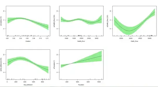
I'm trying to model a relationship between marine debris concentration (item/m^2) with several covariates using GAM with MGCV R package. I found that the concurvity values at worst-case scenario are very high when i checked it. I read on GAM website tutorial that suggests that if a high concurvity value appears, check the partial smooth plot to see if variables with high values have problematic shapes or confidence intervals, and to be careful in making interpretations. is it means that i could trust the model and keep making interpretation a.k.a ignore the concurvity?. Since i think i don't see any problematic shapes of curve and confidence intervals in paratial plot (?). And also, i don't remove the covariate with high concurvity because i think i need them in my model, and they have significance p-value but i'm not really sure about this because of the concurvity values. Big appreciate for an advice and suggestions. Here i attached the code and the plot. Thanks in advance
m1 <- gam(Concentration ~s(Gradient, k =4) + Shore_exposure + Substrate_type +
            Backshore_type + s(DistBN_River, k=5) + s(DistBL_River, k = 4) +
            Dist_Tourism + s(Dist_Settlement, k=4) + s(Population,k=3),
          family='tw', data=debris.data, method="REML")
concurvity(m1, full = TRUE)
          para   s(Gradient) s(DistBN_River) s(DistBL_River) s(Dist_Settlement) s(Population)
worst  0.9915294   0.9732331      0.9788846       0.9920508         0.9951241         0.9969839
summary(m1)

Family: Tweedie(p=1.99)
Link function: log

Formula:
Concentration ~ s(Gradient, k = 4) + Shore_exposure + Substrate_type +
    Backshore_type + s(DistBN_River, k = 5) + s(DistBL_River,
    k = 4) + Dist_Tourism + s(Dist_Settlement, k = 4) + s(Population,
    k = 3)

Parametric coefficients:
                              Estimate Std. Error t value Pr(>|t|)
(Intercept)                  4.8870188  0.6809171   7.177 6.35e-09 ***
Shore_exposureHEADLAND      -0.5363288  0.3923668  -1.367 0.178610
Shore_exposureSTRAIGHT      -0.1624164  0.2160818  -0.752 0.456274
Substrate_typeROCK SLAB     -0.9361547  0.4760029  -1.967 0.055555 .
Substrate_typeSAND          -1.2949689  0.3355633  -3.859 0.000369 ***
Backshore_typeFOREST/TREE   -1.2002933  0.5409765  -2.219 0.031717 *
Backshore_typeGRASS-PASTURE -1.4185890  0.7063872  -2.008 0.050792 .
Backshore_typeGRASS-TUSSOCK -1.1531053  0.6468418  -1.783 0.081552 .
Backshore_typeMANGROVE      -0.3041392  0.7563493  -0.402 0.689549
Backshore_typeSEAWALL       -1.3858871  0.7793002  -1.778 0.082264 .
Backshore_typeSHRUB         -0.6497938  0.6057003  -1.073 0.289220
Dist_Tourism                -0.0005501  0.0000742  -7.413 2.87e-09 ***
---
Signif. codes:  0 ‘***’ 0.001 ‘**’ 0.01 ‘*’ 0.05 ‘.’ 0.1 ‘ ’ 1

Approximate significance of smooth terms:
                     edf Ref.df      F  p-value
s(Gradient)        2.722  2.933 12.277 2.79e-06 ***
s(DistBN_River)    3.650  3.905  3.017  0.01665 *
s(DistBL_River)    2.865  2.975 12.722 4.58e-06 ***
s(Dist_Settlement) 2.835  2.959 13.734 1.73e-06 ***
s(Population)      1.000  1.000  9.308  0.00381 **
---
Signif. codes:  0 ‘***’ 0.001 ‘**’ 0.01 ‘*’ 0.05 ‘.’ 0.1 ‘ ’ 1

R-sq.(adj) =  0.649   Deviance explained = 86.8%
-REML = 133.24  Scale est. = 0.30842   n = 69
