0

Suppose the registrar's office at a college reports 58% of the students live on campus. An intern working in the administration building is unaware of this 58% parameter value. He designs a study in which he will take a random sample of 200 students and estimate the population proportion of all students that live in the college dorms using the resulting sample proportion.

If he were to repeat his study many times, the possible values of the sample proportion would vary by about __ away from the expected value of __, on average.

I understand the first blank is the standard deviation and the second is the mean, but why can't I approximate them using $\mathcal{N}(np, (np(1-p))^.5)$, which is the normal approximation to a binomial distribution? So that I have $\mathcal{N}(116, 6.98)$? So the first blank is 6.98 and the second is 116?
Peter Flom
  • 94,055
  • 35
  • 143
  • 276
Bob John
  • 207
  • 1
  • 5
  • 12
  • 2
    Is this homework? If so, it should have the homework tag. – Peter Flom Feb 21 '13 at 20:54
  • 1
    Ponder this: when you computed 6.98 and 116, did you need to make a Normal approximation to anything? Can you pinpoint where, if anywhere, you actually use a Normal approximation in this answer? – whuber Feb 21 '13 at 22:13
  • 1
    Possible duplicate of [Is the normal distribution a better approximation to the binomial distribution with proportions near or far from 0.5?](https://stats.stackexchange.com/questions/256357/is-the-normal-distribution-a-better-approximation-to-the-binomial-distribution-w) – kjetil b halvorsen Apr 27 '17 at 17:26

2 Answers2

2

The short answer is that you specified the normal approximation to the binomial distribution of the counts and the question is asking about the distribution of the proportions. Since the proportion is just the count divided by the sample size it is an easy conversion from your answer to the correct answer.

Greg Snow
  • 46,563
  • 2
  • 90
  • 159
1

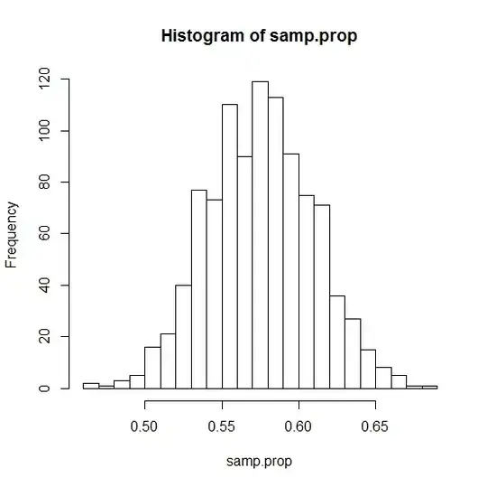
Consider the R code below which shows what the answer is through simulation. You will see that the variance is actually $\dfrac{p(1-p)}{n}$. As the number of samples gets large the distribution of sample proportions is asymptotically normal with distribution $\mathcal{N}(p,\sqrt{\dfrac{p(1-p)}{n}})$, as we would expect. It should be fairly evident why this is the case, but it is helpful to see in the data...

reps <- 1000
p <- .58
pop <- rbinom(size=1,n=10000,p=p)
samp.prop <- rep(0,reps)
for(i in 1:reps){
  samp.prop[i] <- sum(sample(pop,size=200))/200
  }
mean(samp.prop)
var(samp.prop)
p*(1-p)/200
hist(samp.prop,breaks=20)

enter image description here

Dan
  • 99
  • 9
  • 1
    To reduce the risk of miscommunication, I edited your answer to conform to the OP's convention of specifying the standard deviation rather than the variance in the normal distribution. One subtle issue in your answer concerns the sense in which something can "converge" to $p(1-p)/n$ when $n$ itself is the index that is getting arbitrarily large! (You might want to use the language of asymptotics instead of convergence.) – whuber Feb 22 '13 at 17:18