I am trying to troubleshoot model adequacy problems for underdispersed count data (number of correct responses in a simple task; dispersion ratio is 0.3) that I modeled with Conway-Maxwell-Poisson. The residuals of my model look normally distributed, but there is what looks like a nonlinear pattern in the residuals-to-fitted-values plot, at least to my rookie eye. These are the diagnostic plots, as generated by performance::check_model():
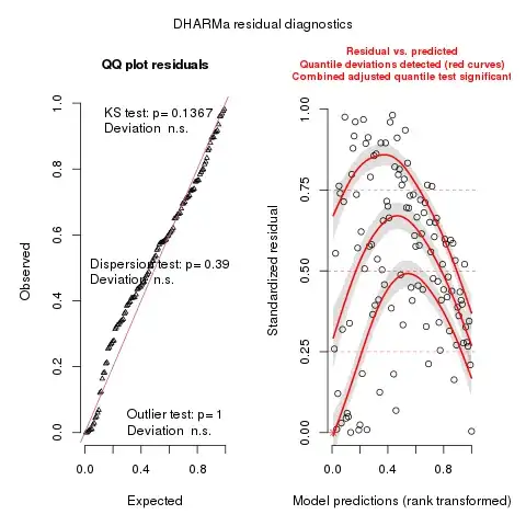
Here is the randomized quantile residual diagnostic plots from DHARMa::simulateResiduals(), as the normality of traditional residuals seems problematic for discrete response variables:
The posterior predictive check doesn't look great either:

My question to the experts out there is whether it looks as bad as I think, and if so, how would you go about troubleshooting? I understand that nonlinearities in the residuals-to-fitted-value plots indicate that some higher order terms is missing or an interaction. When I was exploring the data, I had plotted the log of my response counts to each of my covariates separately to see whether the relationship was linear or required some transformation (tried exponential, quadratic and inverse of my covariates) and I included as many interactions in my max model as it would theoretically make sense and converge. To be honest, it's not always so clear that the raw data was better fitted by a nonlinearization of the covariate. Here is an example with one of the covariates:
I fitted my Conway-Maxwell-Poisson distribution model using glmmTMB::glmmTMB in R with the option family = compois(link = "log"). I had started off with a "max" model with interaction terms and random effect terms, used buildmer::buildglmmTMB() to step backwards and used the likelihood ratio test to arrive at a model that has some interactions with no random effect terms (I know this is arguably not an optimal way of approaching regression modelling....would love ot hear alternatives).
Thanks a ton in advance for any help/advice/hints/words of wisdom!
Gina


