Is this the correct way to check for a heavy-tailed distribution?

Question

I have two distributions and I want to test whether there's an inequality of variances. They're non-normal, so Levene's test is appropriate. The scipy implementation offers three options: test on the mean, the median, and the trimmed mean. The trimmed mean is appropriate for heavy tailed distributions.

My question is, how do I know if my distribution is heavy-tailed? My understanding is that it's heavy-tailed if it's not exponentially bounded. I've tried to check this but I'm not sure if my method is correct. Here's what I did:

1. Converted my data into z-scores so as to standardise it and plotted it.

2. Plotted the exponential distribution function across the range of my data, plotted it.

3. Compared the two visually.

EDIT: I'm here adding some descriptive statistics about my two distributions in response to the comments. This is the raw data, not the z scores.

Distribution 1: 

count    38.000000
mean      1.160140
std       1.281058
min       0.220619
25%       0.451241
50%       0.623582
75%       1.478313
kurtosis  7.57
max       6.719054

Distribution 2: 

count    40.000000
mean      0.887812
std       0.720215
min       0.252508
25%       0.408433
50%       0.617842
75%       1.120488
kurtosis  6.27
max       3.939130

My conclusion is that my distribution is not heavy tailed, but I'm not confident about it. Can anyone advise?

EDIT 2: This is my full data, long form:

Group   entropy
1   6.71905356
1   0.56407487
1   0.738029138
1   0.630035416
1   3.017076375
1   2.510090903
1   0.254787047
1   0.376719953
1   0.456298101
1   0.328258469
1   0.767253283
1   0.641643213
1   2.905235741
1   3.615227362
1   0.244727319
1   2.317604878
1   1.504713298
1   0.999700392
1   0.669730607
1   0.766398132
1   0.449555621
1   0.360902977
1   0.297898424
1   1.399111031
1   0.67895411
1   0.56984134
1   0.536010552
1   2.226602414
1   1.998649951
1   0.220619041
1   0.547186366
1   0.446506256
1   0.495662791
1   0.458900635
0   1.699580285
0   1.017646859
0   0.618058775
0   0.740520854
0   0.558418925
0   0.264262271
0   1.4136416
0   0.538862166
0   2.089605078
0   2.206855803
0   0.494698728
0   0.36284015
0   0.947420619
0   1.515928283
0   0.682302263
0   0.515864165
0   0.400418084
0   0.401584527
0   1.195820577
0   0.544921866
0   0.284516915
0   1.902155181
0   1.095376897
0   0.263003363
0   0.674095659
0   3.939129819
0   0.617625765
0   0.364223021
0   0.355701427
0   0.887284165
0   0.312722361
0   0.570313528
0   0.4107156
0   0.453855313
0   1.441497841
1   1.720034593
1   0.590291826
1   0.444819008
0   0.252508237
0   1.226010557
0   0.526118886
0   1.046928619
0   0.679454156
1   0.617128565

Answer 1

This isn't a complete answer, but the graphs it shows can't be included easily in a comment.

Your summary statistics allow box plots to be drawn and transformations to be tried in exploratory fashion.

Here I note that distribution 1 does have higher variability than distribution 2, as the standard deviations imply. I am not a great fan of tests comparing variances, but they exist. Perhaps a better procedure would be to get a confidence interval for the variance ratio by bootstrapping and see if it contains 1.

I suggest considering working on logarithmic scale.

Either way your sample sizes (38 and 40; Python's default of adding 6 decimal places is curious, but I've seen the same dopeyness in my own favourite software) are small enough that you could post the entire dataset here. Particularly interesting to me is how far the higher variability of distribution 1 is attributable to just a few high values in its tail.

EDIT: The full data allow more to be said. First, as a generic method to get a firmer idea of the variance ratio, I used Stata for bootstrapping. The variance ratio is 3.164 or so, which looks a fair bit bigger than 1, but the 95% confidence intervals all include 1. The normal-based confidence interval doesn't "know" that the variance ratio can't be zero or negative, but set that aside.

. estat bootstrap, all

Bootstrap results                               Number of obs     =         78
                                                Replications      =      10000

      command:  var_ratio entropy
        _bs_1:  r(var_ratio)

------------------------------------------------------------------------------
             |    Observed               Bootstrap
             |       Coef.       Bias    Std. Err.  [95% Conf. Interval]
-------------+----------------------------------------------------------------
       _bs_1 |   3.1638341   .8053801   3.1112753   -2.934153   9.261822   (N)
             |                                       .7221368   12.66759   (P)
             |                                       .7664097   13.44563  (BC)
------------------------------------------------------------------------------
(N)    normal confidence interval
(P)    percentile confidence interval
(BC)   bias-corrected confidence interval

Naturally, other statistics could be used ad hoc to compare variability such as a ratio of SDs or IQRs.

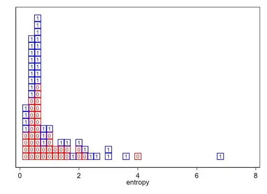
More detailed graphs, a quantile-box plot and a Lego-style histogram, suggest a possible pattern: the two groups have very similar lower values, but group 1 has a longer tail. It's not a matter of a simple additive or multiplicative shift.