Identifying the correlation between a slope and a level

Question

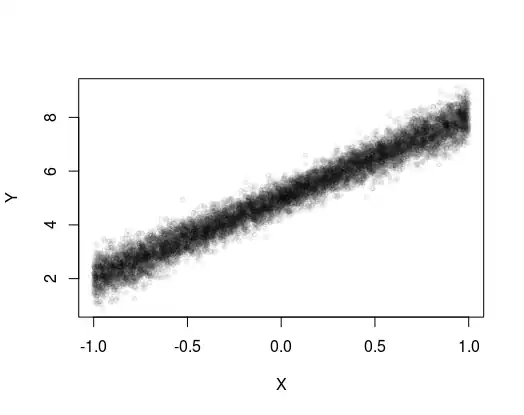
Throughout this post, I assume at least second moments exist. Consider a heterogeneous linear treatment effect model of the form:

$$Y_i = \alpha_i + \beta_i X_i$$

where $\alpha_i, \beta_i$ are potentially arbitrarily heterogenous (in other words, we make no restrictions on heterogeneity in the potential outcomes function, but we do restrict it to be linear). Suppose additionally, that $X_i$ is exogenous/comes from an experiment in the sense that $$X_i \perp \alpha_i, \beta_i$$

Then standard arguments show that $\mathbb E[\alpha_i], \mathbb E[\beta_i]$ are identified by the (population) OLS with $Y_i$ as the outcome and $X_i$ as the covariate. Interestingly enough, we also have that $\mathbb C\mathrm{ov}(\alpha_i, \beta_i)$ is identified under the additional assumption that $X_i$ is symmetrically distributed around its mean. To see why, note that if we define $\tilde X_i = X_i - \mathbb E[X_i]$, we have

$$Y_i^2 \tilde X_i = \alpha_i^2 \tilde X_i + 2\alpha_i \beta_i \tilde X_i^2 + \beta_i^2 X_i^2 \tilde X_i$$

Noting that the first and third term vanish in expectation due to exogeneity and the symmetric distribution of $X_i$, only the third term is left. In particular, we can show that

$$\mathbb C\mathrm{ov}(\alpha_i, \beta_i) = \frac{\mathbb E\left[Y_i^2 \tilde X_i\right]}{2\mathbb E\left[\tilde X_i^2\right]} - \mathbb E[\alpha_i]\mathbb E[\beta_i]$$

where everything above is either directly observed or identified (in particular, the first term on the RHS is half the (population) OLS slope of the regression of $Y_i^2$ on $X_i$). Consider now, the case where I have two outcomes with their own linear-in-treatment potential outcomes:

$$Y_{i,1} = \alpha_{i,1} + \beta_{i,1} X_i$$ $$Y_{i,2} = \alpha_{i,2} + \beta_{i,2} X_i$$

Again, I am assuming that $X_i$ is exogenous in the sense that $X_i \perp \left\{\alpha_{i,j}, \beta_{i,j}\right\}_{j=1}^2$. My question is therefore the following. Can we identify $\mathbb C\mathrm{ov}\left(\alpha_{i,1}, \beta_{i,2}\right)$ in this model without making additional restrictions? The obvious generalization of the above argument does not seem to work here because

$$Y_{i,1} Y_{i,2} \tilde X_i = \alpha_{i,1}\alpha_{i,2} \tilde X_i + \alpha_{i,1}\beta_{i,2} \tilde X_i^2 + \alpha_{i,2}\beta_{i,1} \tilde X_i^2 + \beta_{i,1}\beta_{i,2} X_i^2 \tilde X_i$$

which does not allow us to separate out $\mathbb E\left[\alpha_{i,1}\beta_{i,2} \right]$ and $\mathbb E\left[\alpha_{i,2}\beta_{i,1} \right]$. It seems also that going to higher cross moments involving $Y_{i,1}, Y_{i,2}$ is unlikely to help either, as we end up introducing even more terms that cannot be separately identified. I am wondering if anybody has formally shown that what I am conjecturing here is true.

Edit: By the suggestion in the comments, here is some R code simulating the DGP I have in mind.

set.seed(12351)

# Set up standard normal variables
norm1 <- rnorm(100000)
norm2 <- rnorm(100000)

# Set up covariance matrix between alphas and betas
# Cov(alpha, beta) = 0.05, Var(alphas) = Var(betas) = 0.1
VCV <- matrix(c(0.1, 0.02, 0.02, 0.1), nrow = 2, ncol = 2)

# Draw individual alphas, betas from population where
# E[alphas] = 5, E[betas] = 3, and VCV(alpha, beta) = VCV as above
alphas <- 5 + sapply(1:100000, function(i) (chol(VCV) %*% c(norm1[i], norm2[i]))[1])
betas <- 3 + sapply(1:100000, function(i) (chol(VCV) %*% c(norm1[i], norm2[i]))[2])

# Independently sample Xs
Xs <- 2 * (rbinom(100000, 1, 0.5) - 0.5)

# Define Ys according to individual parameters (alpha, beta) and treatment (X):
Ys <- alphas + betas * Xs

# Run estimators corresponding to the moment equalities from the question
lmod <- lm(Ys ~ Xs)
lmod2 <- lm(Ys^2 ~ Xs)


# Moments for underlying parameters
mean(alphas)
# [1] 4.999713
mean(betas)
# [1] 3.000854
cov(alphas,betas)
# [1] 0.01947037


# As expected, intercept is approximately E[alpha], intercept is
# approximately E[beta], and half the OLS slope of
# Ys^2 ~ Xs minus slope times intercept from Ys ~ X is roughly
# Cov(alphas, betas)
summary(lmod)

# Call:
#   lm(formula = Ys ~ Xs)
# 
# Residuals:
#   Min       1Q   Median       3Q      Max 
# -2.19008 -0.29728  0.00006  0.29893  2.65507 
# 
# Coefficients:
#   Estimate Std. Error t value Pr(>|t|)    
# (Intercept) 4.998635   0.001414    3536   <2e-16 ***
#   Xs          3.001279   0.001414    2123   <2e-16 ***
#   ---
#   Signif. codes:  0 ‘***’ 0.001 ‘**’ 0.01 ‘*’ 0.05 ‘.’ 0.1 ‘ ’ 1
# 
# Residual standard error: 0.447 on 99998 degrees of freedom
# Multiple R-squared:  0.9783,  Adjusted R-squared:  0.9783 
# F-statistic: 4.507e+06 on 1 and 99998 DF,  p-value: < 2.2e-16

as.numeric(lmod2$coefficients[2] / 2 - lmod$coefficients[1] * lmod$coefficients[2])
# [1] 0.01906454

```

Answer 1

A slightly different characterisation of the problem

Instead of these separate variations/errors in $\alpha$ and $\beta$ you could describe the variance of $Y_i$ directly.

A common way (which you see a lot on this site) is to describe a linear function like $$y_i = a+bx_i + \epsilon \quad \text{where} \quad \epsilon \sim N(0,\sigma^2)$$ or

$$y_i|x_i \sim N(a+bx_i,\sigma^2)$$

The above is with normal distributed errors. But you can use other distributions too. In general you could describe the mean and variance for $Y_i$. Conditional on $X_i$ it is often like (the case for homogeneous errors, independent of $x_i$)

$$\begin{array}{rcl} \text{E}[y_i|x_i] &=& \alpha + \beta x_i \\ \text{Var}[y_i|x_i] &=& \sigma^2 \end{array}$$

(In the case of general linear models a description where $\text{Var}[y_i|x_i]$ is a function of $\text{E}[y_i|x_i]$ is also useful)

---

Your case is very similar but now the variance of the error is not a constant $\sigma$ and it depends on $x_i$.

$$\begin{array}{rcl} \text{E}[y_i|x_i] &=& \alpha + \beta x_i \\ \text{Var}[y_i|x_i] &=& \sigma_{\alpha\alpha} + 2 x_i \sigma_{\alpha\beta} + {x_i}^2 \sigma_{\beta\beta} \end{array}$$

where we use $\sigma_{ij}$ to indicate the variance or covariance.

In the case $\alpha = 5, \beta = 3, \sigma_{\alpha\alpha} = \sigma_{\beta\beta} = 0.1, \sigma_{\alpha\beta} = 0.05$ and $X \sim Unif(-1,1)$ it will look like:

It is a linear relationship with heteroscedasticity.

We can estimate the variance and covariance of $\alpha$ and $\beta$ based on this heteroscedastic dependency of the variance of the error (which we might approximate with the residuals).

---

Method of moments

The method that you used is the method of moments. You expressed the expectation of $\tilde X_i Y_i^2$ for the population in terms of coefficients. Then you replace in the expressions the expectation for the population by the average for the sample to obtain estimates of the coefficients.

(In your particular execution there is a small mistake by assuming that the expectation of $X_i^2\tilde X_i$ is zero. This is only true when $X_i$ is distributed symmetrical around zero)

Least squares method

A simpler approach might be to model the expectation of the square of the errors as a linear function of terms of $X_i$ and estimate it with the least squares method applied to the residuals. (It is simpler because it is straightforward and it will help to generalize the problem)

The errors are distributed as:

$$E(\epsilon_i^2) = \text{Var}[y_i|x_i] = \sigma_{\alpha\alpha} + 2 x_i \sigma_{\alpha\beta} + {x_i}^2 \sigma_{\beta\beta}$$

library(MASS)
  
fit <- function(cMu, cSigma, n) {
  ### generate data
  coef <- mvrnorm(n,cMu,cSigma) 
  X <- runif(n,-1,1)
  Y <- coef[,1]+coef[,2]*X
  
  ### model means
  mod <- lm(Y ~ X)
  res <- mod$residuals
    
  ### model covariance tabel
  modr <- lm(res^2 ~ 1 + I(2*X) + I(X^2))
      ### using glm as a slight improvement to lm 
      ### as the variance is not homogeneous but scales with mu
      ### (note that res^2 follows a chi-square distribution 
      ###  for which we have var = 2*mu)
  modr <- glm(res^2 ~ 1 + I(2*X) + I(X^2), 
              family = quasi(link = "identity", variance = "mu"),
              start = coef(modr))  
  ### fitcov 
  fitcov <- mean(X*Y^2)/(2*mean(X^2)) - prod(coef(mod))
  
  ### return result  
  ret <- c(coef(modr),fitcov)
  names(ret) <- c("alpha", "cov", "beta", "fitcov")
  return(ret)
}

### settings
set.seed(1)
n <- 10^4
cSigma <- matrix(c(0.1,0.05,
                   0.05,0.1), 2, byrow = 1)
cMu <- c(5,3)

### generate data and perform fitting
fit(cMu,cSigma, 10^5) 

---

Maximum Likelihood

I guess that you might also maximize the likelihood function (or a quasi-likelihood function if you do not see a particular distribution and stick to a formulation with only known conditional mean and variance).

But I can not find a closed solution for this. It can be done computationally. I leave this as a separate problem as writing a function that solves it might make this answer too cluttered. In addition, I am not sure whether it will be much faster or more accurate than solving it with the method of moments or fitting the square of the residuals.

Generalising

Your problem with two equations can be solved in the same way. Now we have two sets of residuals $r_{1i}$ and $r_{2i}$ whose expectation of the products depend on the covariance of the $\alpha_1$, $\alpha_2$, $\beta_1$ and $\beta_2$.

$$\begin{array}{rcl} \text{E}[r_{1i}r_{2i}|x_i] &=& \sigma_{\alpha_1\alpha_2} + x_i (\sigma_{\alpha_1\beta_2} + \sigma_{\alpha_2\beta_1}) + {x_i}^2 \sigma_{\beta_1\beta_2} \end{array}$$

You have indeed the term $(\sigma_{\alpha_1\beta_2} + \sigma_{\alpha_2\beta_1})$ whose terms can not be separated with this single equation. The dependency of $r_{1i}r_{2i}$ or $y_{1i}y_{2i}$ on $x_i$ is dependent on the sum but not the independent terms.

If you would measure the $y_{1i}$ and ${y_{2i}}$ based on the same correlated $\alpha_1$, $\alpha_2$, $\beta_1$ and $\beta_2$, but with different $x_i$ (say $x_{1i}$ and $x_{2i}$) then you could separate the variables

$$\begin{array}{rcl} \text{E}[r_{1i}r_{2i}|x_i] &=& \sigma_{\alpha_1\alpha_2} + x_{2i} \sigma_{\alpha_1\beta_2} + x_{1i} \sigma_{\alpha_2\beta_1} + x_{1i}x_{2i} \sigma_{\beta_1\beta_2} \end{array}$$

---

For what it is worth, here's a code that would compute the covariances (based on the linear fit of the residual term):

fit2 <- function(cMu, cSigma, n) {
  ### generate data
  coef <- mvrnorm(n,cMu,cSigma) 
  X <- runif(n,-1,1)
  Y1 <- coef[,1]+coef[,2]*X
  Y2 <- coef[,3]+coef[,4]*X
    
  ### model means
  mod1 <- lm(Y1 ~ X)
  res1 <- mod1$residuals
  mod2 <- lm(Y2 ~ X)
  res2 <- mod2$residuals
  
  ### model covariance tabel
  modr <- lm(I(res1*res2) ~ 1 + I(X) + I(X^2))
  
  ### return result  
  ret <- c(coef(modr))
  names(ret) <- c("alpha-alpha", "alpha-beta", "beta-beta")
  return(ret)
}



### settings
set.seed(1)
n <- 10^4
                  # a1, b1 , a2,  b2
cSigma <- matrix(c(0.10,0.05,0.10,0.10,
                   0.05,0.10,0.10,0.10,
                   0.10,0.10,0.40,0.20,
                   0.10,0.10,0.20,0.40), 4, byrow = 1)
       # a1 , b1 , a2 , b2
cMu <- c( 5,   3,   5,   3)

### generate data and perform fitting
fit2(cMu,cSigma, n)

Answer 2

Let me not answer the question exactly as I posed it, but to answer a very related question (and in fact, the question I am interested in in the first place). Suppose we have potential outcomes $Y_1(X), Y_0(X)$, and suppose that for each individual has a default level of $X$, say $X_d$, in the absence of experimental intervention. Suppose that the experimenter can shock $X$ from its default level by some randomized quantity $\varepsilon$ so that locally, the experimenter can (at least in principle) use an experiment to measure any quantity taking the form $$\frac{d g(Y_1(X_d + \varepsilon), Y_2(X_d + \varepsilon))}{d\varepsilon}\bigg |_{\varepsilon = 0}$$ for some pre-specified function $g(Y_1, Y_2)$. Translating my original question into this framework, the claim that $\mathbb E[\alpha_i\beta_i]$ (and hence $\mathbb C\mathrm{ov}(\alpha_i, \beta_i)$) is identified follows from the observation that taking $g(Y_1, Y_2) = \frac12 Y_1^2$ gives $$\frac{d g(Y_1(X_d + \varepsilon), Y_2(X_d + \varepsilon))}{d\varepsilon}\bigg |_{\varepsilon = 0} = \underbrace{Y_1}_{"\alpha_i"}\cdot \underbrace{\frac{d Y_1}{d\varepsilon}\bigg|_{\varepsilon = 0}}_{"\beta_i"}$$

where I am being a bit loose with notation on the RHS above. Similarly, when we take $g(Y_1, Y_2) = Y_1 Y_2$, we have $$\frac{d g(Y_1(X_d + \varepsilon), Y_2(X_d + \varepsilon))}{d\varepsilon}\bigg |_{\varepsilon = 0} = \underbrace{Y_1 \frac{d Y_2}{d X}}_{"\alpha_{i,1}\cdot \beta_{i,2}"} + \underbrace{Y_2 \frac{d Y_1}{d X}}_{"\alpha_{i,2}\cdot \beta_{i,1}"}$$

The question now, is whether the individual terms on the RHS above can be separately identified (instead of just identifying their sum) using some function $g$. Since we just showed that their sum can be identified, this is equivalent to asking if there exists some $g$ such that

$$\frac{d g(Y_1(X_d + \varepsilon), Y_2(X_d + \varepsilon))}{d\varepsilon}\bigg |_{\varepsilon = 0} = \frac{\partial g}{\partial Y_2}\frac{d Y_2}{dX} + \frac{\partial g}{\partial Y_1}\frac{d Y_1}{d X} = Y_1 \frac{d Y_2}{d X} - Y_2 \frac{d Y_1}{d X}$$

at all $Y_1, Y_2$. But this requires $g$ to satisfy the following system of PDE

$$\frac{\partial g}{\partial Y_1} = -Y_2,\quad \frac{\partial g}{\partial Y_2} = Y_1$$

Such a $g$ cannot exist on any neighborhood. To see why, fix some point $(a,b)$, and consider $g(a,b)$ compared to $g(a+\delta, b + \delta)$ for any $\delta > 0$. WLOG, we can normalize $g(a,b) = 0$. Using the PDE system above, we can try to evaluate $g(a+\delta,b+\delta)$ two different ways. First, we could first integrate along the first dimension and then integrate along the second dimension to get $g(a+\delta,b+\delta) = -\delta b + \delta (a + \delta)$. Second, we could first integrate along the second dimension and then integrate along the first to get $g(a+\delta,b+\delta) = - \delta(b + \delta) + \delta a$. Setting these two expresssings for $g(a+\delta,b+\delta)$ and simplifying, we arrive at the contradiction $\delta = - \delta$. I am not sure that this completely rules out any way of identifying the cross-equation correlations separately, but it certainly suggests that no treatment-effect based approach on its own will work.