I looked quickly at the link and didn't see the most direct explanation, but might have skimmed too fast. Expanding "$P(B)$" in this way uses the law of total probability. The idea is that if you have a partition of the sample space, the we can find $P(B)$ by summing up the probability parts of $B$ found in each of the partitions. A partition just means that we have split the sample space in such a way that each point can be found in exactly one of the partitions or groupings.
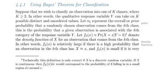
In your case, each observation is assumed to be in exactly one of the $K$ classes, i.e the classes are your partition. They say there is a discrete random variable $Y$ which represents membership to the $k$th class. The event that an observation belongs to the kth class is then simply $\{Y=k\}$.
The law of total probability can be shown as follows for arbitrary $B \subseteq \Omega$, where $\Omega$ is the sample space. (or more formally $B \in \mathcal{F}$, where $\mathcal{F}$ is the appropriate sigma algebra).
\begin{align*}
P(B) &= P(B \cap \Omega)\\
&= P(B \cap (\cup_{i=1}^K\{Y =i\}))\\
&= \sum_{i=1}^KP(B\cap \{Y =i\})\\
&= \sum_{i=1}^K P(B|\{Y =i\})P(\{Y =i\})\\
\end{align*}
The third line follows because the events are disjoint (no overlap between the classes) and the last line follows from the multiplicative rule of probability.
Notice that $P(Y = i)$ is just the weight $\pi_i$ for class i. Similarly, in your text they denote $P(X=x|Y=k) = f_k(x)$ to be the probability of $X=x$ given it is in class K if $X$ is discrete or the probability density of $X$ given membership in class K if it is continuous. (Not shown, but the law of total probability can be extended to the continuous case when we are working with densities).
Now why do we do this? The answer is because it is easier in the set up given by the problem. The classifier model assumes a density for each class $f_i(x)$, but not a density for the observations in general, $f(X=x)$. So to figure out the density $f(X=x)$ it is much easier to split this up into the classifier densities and the law of total probability gives us a way to do that, by simply summing the classifier densities weighted by how likely they are to occur. This technique is so useful and common that in many elementary probability texts Bayes rule is expressed directly in the partition form (usually for say partition into event $A$ and its complement, $A^c$.).

