Using $\chi^2$-Distance for Histogram-Comparison with 0-Valued Elements leads to NaNs

Question

I want to compare two histograms by using the $\chi^2$-distance. There is a definition in the OpenCV-library. Also this question gives a lot of insight about this distance-metric. Because i didn't find a suitable function in MATLAB i implemented it like this:

function [dist] = chi2_distance(hist1, hist2)
    dist = sum((hist1 - hist2).^2 ./ hist1);
end

which follows the definition found in OpenCV:

$$ d(H_1, H_2) = \sum_i^n \frac{(H_1(i) - H_2(i))^2}{H_1(i)} $$

with $n$ being the number of elements in the histogram. However, if there is a $0$-valued element in $H_1$ this formula will yield NaN because dividing by $0$ yields $\infty$.

Is there an alternative formulation or some modification i should perform on the given formula to make it work?

Answer 1

Histograms, KDEs and ECDFs for comparing a sample to a distribution. Often (sample) empirical CDFs (ECDFs) give a better idea of the CDF of a population than histograms do at suggesting the density function. [To make an ECDF of a sample of size $n,$ sort the data, start at $0$ height at the left, increment upwards by $1/n$ at each sorted data point, ending at $1$ on the right. If there are $k$ observations tied at a value, then increment by $k/n$ at that value.]

Here is an example of a histogram and an ECDF of $n=200$ observations from $\mathsf{Beta}(3,5).$

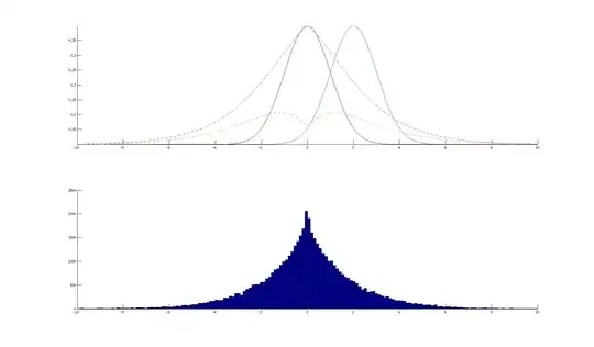
At left is the histogram of the data, a kernel density estimator (KDE) based on the data, and the density function of $\mathsf{Beta}(3,5)$ (dotted lines) At right is the ECDF of the data along with the CDF of $\mathsf{Beta}(3,5).$

set.seed(1116)
x = rbeta(1900, 3,5)
par(mfrow=c(1,2))
 hist(x, prob=T, br=15, col="skyblue2")
  lines(density(x), col="red")
  curve(dbeta(x, 3,5), add=T, lty="dotted", lwd=2)
 plot(ecdf(x), col="skyblue2")
  curve(pbeta(x, 3,5), add=T, lty="dotted", lwd=2)
par(mfrow=c(1,1))

Compared with the KDE, the histogram gives only a rough approximation of the density function. The KDE can be regarded as a sort of 'smoothed histogram', but it is computed independently of the histogram.

The ECDF (blue) gives a close approximation of the CDF of the population (dotted).

Comparing two samples. Here we compare samples of size $n=200;$ one from $\mathsf{Beta}(3,5)$ and one from $\mathsf{Beta}(4,4).$

First, we compare histograms of the two samples.

set.seed(2020)
x1 = rbeta(200, 3,5);  x2 = rbeta(500, 4,4)
par(mfrow=c(1,2))
 hist(x1, prob=T, col="skyblue2", main="BETA(3,5)")
 hist(x2, prob=T, col="wheat", main="BETA(4,4)")
par(mfrow=c(1,1))

By visual inspection, the histograms show some difference in shape. Keeping in mind the Comment by @whuber, you can see whether your chi-squared test on bin counts finds a significant difference. Your idea of ignoring a bin with 0 counts may work OK. I am not enthusiastic about this test and will leave the computation to you.

A straightforward chi-squared contingency table of bin counts may be better. In R, you can get bin counts by using a non-plotted 'histogram's. [You'd need to check that the two histograms use exactly the same bins. Look at hist(x1, plot=F)$breaks and similarly for x2.]

f1 = hist(x1, plot=F)$counts;  f1
[1]  7 29 31 49 39 29 11  4  1
f2 = hist(x2, plot=F)$counts;  f2
[1]   4  17  45  78 128  96  75  39  16   2
TBL = rbind(c(f1,0), f2); TBL
   [,1] [,2] [,3] [,4] [,5] [,6] [,7] [,8] [,9] [,10]
      7   29   31   49   39   29   11    4    1     0
f2    4   17   45   78  128   96   75   39   16     2

chisq.test(TBL)

        Pearson's Chi-squared test

data:  TBL
X-squared = 72.609, df = 9, p-value = 4.678e-12

Warning message:
In chisq.test(TBL) : Chi-squared approximation may be incorrect

R can provide a simulated P-value when low cell counts call the validity of the chi-squared distribution into doubt. The small P-value indicates the two histograms have significantly different cell counts. [Without simulation, you might try combining the first two bins and the last two bins, in order to avoid small counts.]

chisq.test(TBL, sim=T)

        Pearson's Chi-squared test 
        with simulated p-value 
        (based on 2000 replicates)

data:  TBL
X-squared = 72.609, df = NA, p-value = 0.0004998

The Kolmogorov-Smirnov test is a reasonably good way of determining whether two samples come from the same population. The test statistic $D$ is the maximum vertical distance between the two ECDFs. A Kolmogorov-Smirnov test comparing ECDFs also finds a highly significant difference.

plot(ecdf(x1), col="blue")
lines(ecdf(x2), col="brown") 

ks.test(x1, x2)

        Two-sample Kolmogorov-Smirnov test

data:  x1 and x2
D = 0.301, p-value = 1.145e-11
alternative hypothesis: two-sided

Finally, a nonparametric two-sample Wilcoxon (rank sum) test, finds a highly significant difference between the two samples x1 and x2. Because the two samples are of somewhat different shapes, this test cannot be interpreted as showing a difference between the two population medians. Instead we can say that x2 'stochastically dominates x1.

Roughly speaking, this means that values from $\mathsf{Beta}(4,4)$ tend to be larger than values from $\mathsf{Beta}(3,5).$ More precisely, the ECDF (brown) of the second sample lies below and to the right of the ECDF (blue) of the first sample.

wilcox.test(x1, x2)

        Wilcoxon rank sum test with continuity correction

data:  x1 and x2
W = 30163, p-value = 2.263e-16
alternative hypothesis: true location shift is not equal to 0