(1) Let $S = \sum_i X_i.$ Then $Var(S) = \sum_i Var(X_i) = 100(4) = 400$, by independence,
assuming your notation means $Var(X_i) = 4.$
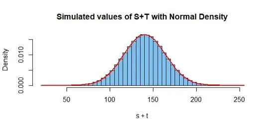
Similarly, $T = \sum_i Y_i$ has $Var(T) = 20(9)= 180.$ So assuming the $X_i$ are independent of the $Y_i,$ you have $Var(S+T) = 400+180 = 580.$
(2) By contrast, if $X \sim \mathsf{Norm}(\mu=1, \sigma=2),$ you have $Var(100X)$
$= 100^2Var(X)$ $= 40000.$ And if, independently $Y \sim\mathsf{Norm}(\mu=2,\sigma=3),$ then $Var(20Y) = 20^2Var(Y)$ $= 400(9)$ $= 3600.$
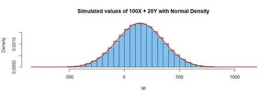
Then $Var(100X + 20Y) = 40000 + 3600 = 43600.$
Simulation of (1): Notice that the third argument of rnorm is the
population standard deviation. With a million iterations, one can
expect about two significant digits of accuracy for variances, which
have squared units.
set.seed(1114)
s = replicate( 10^6, sum(rnorm(100, 1, 2)) )
t = replicate( 10^6, sum(rnorm(20, 2, 3)) )

mean(s); mean(t);  mean(s+t)
[1] 100.0397    # aprx E(S) = 100(1) = 100
[1] 40.0168     # aprx E(T) = 20(2_ = 40
[1] 140.0565    # aprs E(S+T) = 140

var(s);  var(t);  var(s+t)
[1] 398.7767   # aprx Var(S) = 400
[1] 180.19     # aprx Var(T) = 180
[1] 579.8212   # aprx Var(S+T) = 580

hdr = "Simulated values of S+T with Normal Density"
hist(s+t, prob=T, br=50, col="skyblue2", main=hdr)
 curve(dnorm(x, 140, sqrt(580)), add=T, col="red", lwd=2)
(2) Simulated:
set.seed(2020)
x = rnorm(10^6, 1, 2)
px = 100*x
y = rnorm(10^6, 2, 3)
py = 20*y
sp = px + py
mean(px);  mean(py);  mean(sp)
[1] 100.1081    # aprx E(100X) = 100(1) = 100
[1] 39.92436    # aprx E(20Y) = 20(2) = 40
[1] 140.0325    # aprx(E(100X + 20Y) = 100 + 40 = 140
var(px);  var(py);  var(sp)
[1] 39936.98    # aprx Var(100X) = 10000(4) = 40000
[1] 3601.973    # aprx Var(20Y) = 400(9) = 3600
[1] 43521.24    # aprx Var(100X + 20y) = 43600

hdr = "Simulated values of 100X + 20Y with Normal Density"
hist(sp, prob=T, br=50, col="skyblue2", main=hdr)
 curve(dnorm(x, 140, sqrt(43500)), add=T, col="red", lwd=2)