I love graphical displays. Here are two that illustrate the right hand side of the law of total variance nicely. First, some code for a linear but heteroscedastic regression.
set.seed(12345)
nsim = 100
X = runif(nsim, 40,120)
Y = 1 + 0.3*X + rnorm(nsim, 0, 0.15*X)
Cond.Mean = 1 + 0.3*X # Conditional Mean
Cond.SD = 0.15*X # Conditional Standard Deviation
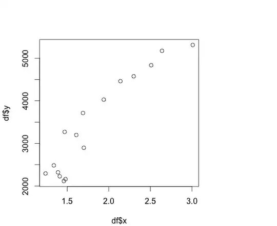
plot(X,Y, main = "Illustrating Variance of Conditional Mean")
abline(1,.3)
rug(Cond.Mean, side=2)
The resulting graph is as follows:
The vertical spread of the of the data ticks (the "rug") on the vertical axis represents the variance of the conditional mean values, or $Var_X[E[Y|X]]$. Notice that this range is a lot smaller than the overall vertical data range, which represents $Var[Y]$.
To visualize the mean of the conditional variance, add the $\pm \sigma_{Y|X}$ bands to the scatter as follows:
plot(X,Y, main = "Illustrating Mean of Conditional Variance")
abline(1,.3)
abline(1,.15, lty=2)
abline(1,.45, lty=2)
rug(X)
The resulting graph is as follows:
Now, for every $x$ value on the "floor" (the "rug"), there is a different vertical spread of potential $Y$ values, as indicated by the $\pm \sigma_{Y|X}$ bands. Each of these spreads represents (via squaring) a conditional variance $Var[Y|X=x]$. The average of all these conditional variances is equal to the other term on the right side, $E_X[Var[Y|X]]$.
You can attempt to verify the equality using
var(Y)
var(Cond.Mean) + mean(Cond.SD^2)
but there is a lot of finite-sample variability, so the results are not that close for this small simulation. On the other hand, if you keep the same seed and change nsim to 20000000, the results are very close, 204.05 and 204.01.

