What does " Y axis" mean in continuous probability distribution?

Question

I understand X-axis means values of the random variable X, but I wonder how I should call or think of the Y-axis. If I find a specific value of the random variable in a continuous probability distribution, the probability is zero. As far as I understand the Y-axis means relative frequencies but I am not sure how it is properly called and what it means. To me, the Y-axis is kind of meaningless.

Answer 1

There are two common ways to represent a probability distribution, the probability density function (PDF) and cumulative distribution function (CDF). I suspect you're wondering most about the former. For the latter, the distribution is plotted as cumulative from zero to one, so the y-axis is the sum of the distribution up to a given value of x.

For a probability density function, there's a big hint in the name: it's a density. You're right, though, that we don't often think of this Y-axis as all that important. PDFs are plotted all the time without any labeled Y-axis. But if you were to label it, you would read it as a density: the sum probability of some unit range in X. You can consider the range in some infinitely narrow range of X, but that infinitely narrow range still has units in X to give a density.

Answer 2

I suppose you have a moderately large or large random sample from a continuous distribution, and that you want to make a plot of the data that suggests the shape of the population distribution.

Then a starting point would be to make a 'density' histogram in which the total area of all bars adds to unity $(1).$ [Similarly, the total area beneath a density curve is unity.]

Here is a sample of size $n = 1000$ from the slightly right-skewed gamma distribution, $\mathsf{Gamma}(\mathrm{shape}=5,\mathrm{rate}=0.1),$ which has $\mu = 50, \sigma^2 = 500, \sigma= 22.36,$ as simulated in R.

    set.seed(2020)
    x = rgamma(1000, 5, 0.1)
    summary(x);  sd(x)
       Min. 1st Qu.  Median    Mean 3rd Qu.    Max. 
      6.637  33.938  46.370  49.928  61.942 163.680 
    [1] 22.61689   # sample SD

    hist(x, prob=T, br=20, col="skyblue2")
     lines(density(x), lwd=2, col="orange")
     curve(dgamma(x, 5, .1), add=T, lwd=2, lty="dotted")

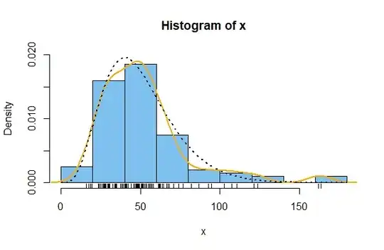
In the figure, the dotted black curve is the density curve (PDF) of $\mathsf{Gamma}(5, 0.1),$ the histogram bars are plotted on a density scale, and the orange curve is the default 'kernel density estimator' (KDE) in R. For a sample of size as large as $n=1000$ it is not surprising that the histogram is a reasonably good fit to the population PDF or that the KDE is very nearly the same as the PDF.

By contrast, if I look at only the first 100 of the $n=1000$ observations above, the histogram and the KDE still approximate the PDF, but not quite as well. Individual tick marks show the exact positions of the 100 points.

    set.seed(2020)
    x = rgamma(100, 5, 0.1)
    summary(x);  sd(x)
     Min. 1st Qu.  Median    Mean 3rd Qu.    Max. 
    15.92   33.50   47.82   51.76   61.39  163.68 
    [1] 27.4087
    hist(x, prob=T, ylim=c(0,.02), col="skyblue2")
     rug(x)
     lines(density(x), lwd=2, col="orange")
     curve(dgamma(x, 5, .1), add=T, lwd=2, lty="dotted")

Note: For small samples, it is feasible to sort the data into appropriate intervals and draw the corresponding histogram by hand, but making a useful KDE is probably best left to software.

Answer 3

Probability density is a density, and may be understood as such.

Although this way of thinking is touched on in other answers, and at greater length in other threads, I find it helpful when trying to teach the topic, and to build on what people should already know about density generally and indeed long since.

Thus in (high school?) physics or other subjects, people should have met density meaning mass per unit volume. In ecology, epidemiology, demography, geography and many social sciences, population density is number of people (or organisms) per unit area. The same idea is easily applied to counting facilities in an area $-$ or along a route, say the number of Starbucks along a road inside a city.

Density has a reciprocal, which is often as interesting or useful. The reciprocal of population density is area per person or organism. The reciprocal of density along a line is the typical distance between objects, both being captured in statements such as there being one Starbucks on average every 200 m.

I can think of another example that is perhaps esoteric, but you should have no difficulty grasping it: drainage density is total length of streams in a region (often, but not necessarily, a basin, catchment or watershed) divided by the area of that region. (Small print: measuring the length of a wiggly line is far from obvious.)

With a little abstraction we can identify the family resemblance as how much stuff there is in a given space.

Time to focus on a concrete example:

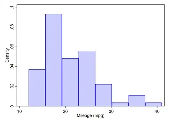
This is close to default as a common-or-garden histogram in my usual statistical environment. It shows a variable, miles per gallon for a bundle of cars, on the horizontal or $x$ axis and has a (probability) density scale on the vertical or $y$ axis.

Now comes the numerical crunch in three parts:

1. The total probability is 1 and is given by the total area of the bars.

2. The range of the variable on the $x$ axis is about 40 (miles per gallon). Rough mental calculations are fine here.

3. So for that to happen the average height of the bars must be about 1/40, because we can think of an implied rectangle with area given by

average height of bars $\times$ range on $x$ axis $\equiv$ 1.

So, the average height of bars should be about 0.025, which checks out when we look at the graph. (There may be a little arm-waving at this point, but usually the listener can see that the number has the right order of magnitude.)

The units (of measurement) of probability density follow from the fact that probability has no units, so

units of probability density $\quad \equiv \quad$ 1 / units on $x$ axis

Here the units are simple, gallons per mile, but that is often not so.

Clearly, the story gets more complicated, but not different in principle, if talking about the bivariate or multivariate density of two or more variables considered together.

What doesn't help here is (so far as I can see) an almost universal habit of never specifying units of measurement on a probability density axis. There seem to be three reasons for that:

1. They would often just look odd. Thus hydrologists and many others get used to think of river discharge in cubic metres per second (so $\text{m}^3 \text{s}^{-1}$), but they might blench at being told that probability density for discharge has units $\text{m}^{-3} \text{s}$. (Using non-metric rather than metric units doesn't help.)

2. The units for probability density are just implicit as the reciprocal of the units on the $x$ axis.

3. Nobody else does it, so why should we?

David Finney (1917$-$2018) wrote a splendid article on dimensions in statistics. You may have access to https://www.jstor.org/stable/2346969

I've also found even that people whose other education was strong in mathematics or physical science don't automatically think about what they are doing in statistics in terms of dimensions and units of measurement (even though the point does arise, e.g. in explaining why the standard deviation can be easier to think about than the variance). In particular, frequent puzzlement that a density exceeds 1 somewhere is eased by underlining that probability density usually has quite different units from probability itself.

Answer 4

Just to make it clear with an equation, the probability density function (PDF) $f_X(x)$ of a random variable $X$ is defined as:

$$ dP_X(x) \equiv f_X(x) dx,$$

where $dP_X(x)$ is the infinitesimal probability that the random variable $X$ takes the value $x$ and $dx$ is a differential of the random variable $X$. In other words, the value of the PDF $f_X(x)$ multiplied by $dx$, which is the infinitesimal area under the curve of your plot at $X = x$, is equal to the infinitesimal probability $dP_X(x)$ that the random variable takes the value $X = x$.

You can extend this idea taking $X$ in some range: $a \leq X \leq b$, then the probability to find the random variable $X$ in this interval is:

$$ P_X(a \leq X \leq b) = \int_{a}^b f_X(x) dx,$$

i.e., the area under the curve $f_X(x)$ from $x = a$ to $x = b$.

Basically, we can understand the PDF like an intensive expression or a density of the probability: it gives the probability per unit of the random variable. For example, it is analogous to the concept of mass density in physics, which is defined as mass per unit volume. In order to find the mass, we need to multiply the density by a volume. Here, in order to find the probability we need to multiply the PDF by a range of the random variable.

Answer 5

PDF is the derivative of CDF, i.e., the rate of CDF's change, just like speed is the derivative of moving distance. When you are driving a car, at any particular time moment the passing distance is zero, but the speed (i.e. the rate of the distance's change) is not zero. Do you think that speed is a meaningful measure ?