What can Ido if I get patterns in residuals vs predicted values using `lme4::glmer()` with a GAMMA distribution?

Question

I want to model a response variable (y) as a function of two explanatory variables (x and z). y are concentration measures of a physiological parameter of the human body with a worldwide accepted method (method A). x is a novel method (method B) that might be alternative since it is much cheaper. However, it is thought that method B is more or less accurate depending on the time (z) that the equipment needed is used. So, my goal is to test the significance of x and z to accurately measure y. I have 6 individuals (ID: A,B,C,D,E,F). Below I show the relationship between x and y:

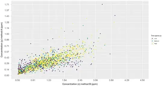
*Note: here I categorized Z for illustration purposes, but z, as x, is numerical, ranging from 1 (hr) to 7 (hr).

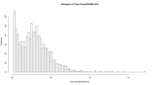
Given that my response variable has a sharp non-normal distribution, that the variance increases as x increases, and that I have several individuals but I am not interested in differences among individuals, I though on GLMM with a GAMMA distribution to test the significant effect of x and z for explaining y.

I run GLMMs with a gamma distribution and using the log link.

## Setting random structure ####
mod1<-glmer(Y~ 1 + (1|ID),data = df, family=Gamma(link=log)) 
mod2<-glmer(Y~ 1 + (X|ID),data = df, family=Gamma(link=log)) 
AIC(mod1,mod2)

## Setting fixed structure ####
mod1<-glmer(Y~ 1 + (X|ID),data = df, family=Gamma(link=log), control = glmerControl(optimizer ="Nelder_Mead")) 
mod2<-glmer(Y~X + (X|ID),data = df, family=Gamma(link=log), control = glmerControl(optimizer ="Nelder_Mead")) 
mod3<-glmer(Y~X + Z + (X|ID),data = df, family=Gamma(link=log), control = glmerControl(optimizer ="Nelder_Mead")) 
mod4<-glmer(Y~X + X:Z +  (X|ID),data = df, family=Gamma(link=log), control = glmerControl(optimizer ="Nelder_Mead")) 

r.squaredGLMM(mod4)[1,c(1,2)]

mod.list <- list(mod1,mod2,mod3,mod4)
model.sel<-model.sel(mod.list, rank="AIC",extra=c(r2=function(x) round(r.squaredGLMM(x)[1,c(1,2)],2)))

To test if x and z are significant I compared models by AIC.

model.sel

Model selection table 
  (Intr) ns(VDB.V13,3)    n.V13 cnd((Int)) dsp((Int)) cnd(ns(VDB.V13,3)) cnd(n.V13:VDB.V13) r2.R2m r2.R2c    class   control ziformula dispformula     random df   logLik     AIC  delta weight
3 -2.567             + -0.04178                                                               0.66   0.71 glmerMod gC(Nl_Md)                          VD.V1|I  9 2017.580 -4017.2   0.00      1
2 -2.645             +                                                                        0.65   0.70 glmerMod gC(Nl_Md)                          VD.V1|I  8 2006.875 -3997.7  19.41      0
4                                   -2.661          +                  +                  +   0.66   0.76  glmmTMB                  ~0          ~1 c(VD.V1|I)  9 2001.622 -3985.2  31.92      0
1 -1.559                                                                                      0.00   0.36 glmerMod gC(Nl_Md)                          VD.V1|I  5 1682.428 -3354.9 662.31      0
Abbreviations:
control: gC(Nl_Md) = ‘glmerControl(Nelder_Mead)’
Models ranked by AIC(x) 
Random terms: 
VD.V1|I = ‘VeDBA.V13AP | ID’
c(VD.V1|I) = ‘cond(VeDBA.V13AP | ID)’

My problem comes when I observe the residual patterns vs predicted values since I think there are clear patterns. Here I don't show the distribution of the residuals since if I understand correctly, a normal distribution of them is not needed.

Does anyone know what I could do? Any proposal? I did not share the data because is too long (n=2027).

Thanks in advance

Head of my dataframe:

   ID          Y          X Z
1   A 0.34136077 1.55682000 2
2   A 0.05124066 0.05766000 2
3   A 0.05901189 0.05125333 3
4   A 0.05213855 0.05766000 2
5   A 0.05437708 0.05125333 3
6   A 0.08433229 0.05766000 3
7   A 0.03618396 0.04484667 3
8   A 0.03622474 0.05766000 1
9   A 0.18244336 0.05125333 3
10  A 0.03625487 0.03844000 2
11  A 0.03840890 0.04484667 3
12  A 0.04235018 0.03844000 3
13  A 0.03862926 0.03844000 3
14  A 0.03749647 0.02883000 2
15  A 0.04395015 0.03844000 2
16  A 0.04040225 0.04805000 2
17  A 0.04419507 0.05766000 3
18  A 0.33186947 2.53704000 1
19  A 0.31986092 0.74958000 1
20  A 0.08127853 0.05766000 1
")

Procedure followed according to the proposal of JTH

mod1<-glmer(Y~ 1 + (X|ID),data = df, family=Gamma(link=log), control = glmerControl(optimizer ="Nelder_Mead")) 
mod2<- glmer(Y~ ns(X, 4)  + (X|ID),data = df, family=Gamma(link=log), control = glmerControl(optimizer ="Nelder_Mead")) 
mod3<-glmer(Y~ ns(X, 4) + Z + (X|ID),data = df, family=Gamma(link=log), control = glmerControl(optimizer ="Nelder_Mead")) 
mod4<-glmer(Y~ X:Z + ns(X, 4) +  (X|ID),data = df, family=Gamma(link=log), control = glmerControl(optimizer ="Nelder_Mead")) 
mod5<-glmer(Y~ ns(X, 4):Z +  (X|ID),data = df, family=Gamma(link=log), control = glmerControl(optimizer ="Nelder_Mead")) 
AIC(mod1,mod2,mod3,mod4,mod5)

The results are next:

r.squaredGLMM(mod4)[1,c(1,2)]

mod.list <- list(mod1,mod2,mod3,mod4)
model.sel<-model.sel(mod.list, rank="AIC",extra=c(r2=function(x) round(r.squaredGLMM(x)[1,c(1,2)],2)))

model.sel

        Int ns(X)            Z       Z:X Z:ns(X)  r2m  r2c df   logLik       AIC     delta       weight
4 -2.827029     +              0.1871558         0.65 0.69 10 320.9342 -621.8684   0.00000 1.000000e+00
2 -2.660326     +                                0.48 0.54  9 289.8442 -561.6884  60.17996 8.552394e-14
3 -2.660204     + 0.0001000814                   0.48 0.54 10 289.8443 -559.6886  62.17976 3.146559e-14
5 -2.220731                                    + 0.04 0.72  9 259.3610 -500.7219 121.14643 4.936132e-27
1 -1.377842                                      0.00 0.27  5 246.9520 -483.9039 137.96446 1.100015e-30

The plot of my residuals vs predicted values is this now:

Although the patterns have been sharply reduced, I suspect there is still some heteroscedasticity. However, I can't remove it.