1

I have always been convinced that maximum likelihood estimation is a very nice method to estimate the parameter of a probability distribution, since the first day I learn about it. However, when I was thinking about the intuition behind Fisher information, I ran into this What kind of information is Fisher information? and found myself a little bit confused. It says we can think Fisher information of a way to measure the curvature of the log likelihood, if we write it as $$ \begin{aligned} I(\theta^{\star})&=-[\mathbb{E}_{X\sim\theta^{\star}}\frac{\partial^2}{\partial\theta^2}\log f(X;\theta)]\mid_{\theta=\theta^{\star}} \end{aligned} $$ Adding some conditions, we may interchange integration and differentiation to get $$ \begin{aligned} I(\theta^{\star})&=-[\frac{\partial^2}{\partial\theta^2}\mathbb{E}_{X\sim\theta^{\star}}\log f(X;\theta)]\mid_{\theta=\theta^{\star}} \end{aligned} $$ Then we can interpret $I(\theta^{\star})$ as the curvature of the expected log likelihood around $\theta^{\star}$ when data actually follows $\theta^{\star}$.

So here comes my question: is the expected log likelihood $\mathbb{E}_{X\sim\theta^{\star}}\log f(X;\theta)$ (a function of $\theta$) maximized at $\theta=\theta^{\star}$? If not, I think it may weaken the "reasonability" of MLE. Is this just my needless worry? Or it's just that I get something wrong about Fisher information.
kjetil b halvorsen
  • 63,378
  • 26
  • 142
  • 467
  • 1
    See also https://stats.stackexchange.com/questions/92097/why-maximum-likelihood-and-not-expected-likelihood/449782#449782 – kjetil b halvorsen Sep 06 '20 at 13:18
  • 1
    Yes, the expected log-likelihood is maximised at the true value $\theta^*$. This is why the Kullback-Leibler divergence is always non-negative. – Xi'an Sep 06 '20 at 15:05
  • Furthermore, under regularity conditions, the expected score$$\mathbb{E}_{X\sim\theta^{\star}}\left[\frac{\partial}{\partial\theta}\log f(X;\theta)\right]$$is also equal to $0$ when $\theta=\theta^*$. – Xi'an Sep 06 '20 at 15:09
  • 1
    @Xi'an, I suppose the answer I'm looking for is exactly what you say about Kullback-Leibler divergence! Besides, I appreciate all those insights provided by other comments and answers. – Chris Cloud Sep 07 '20 at 02:33

1 Answers1

1

As an illustration, consider trying to estimate binomial $p$ with a known number $n$ of Bernoulli trials of which $x$ turn out to be successes. First, use small $n = 10,$ so that the MLE $\hat p = x/n$ may not be very accurate.

The likelihood function is the PDF considered as a function of $p,$ for observed data. Let's use R to plot the likelihood function for $x =4.$ likelihood function:

x = 4;  n = 10;  p=seq(.1, .9, by = 0.001)
like = dbinom(x, n, p)
plot(p, like, type="l", lwd=2)
abline(h=0, col="green2")

mle = mean(p[like == max(like)])  #'mean' in case of ties with discrete p
mle
[1] 0.4
abline(v = mle, col="orange")

It seems clear that the likelihood function attains its maximum value at $\hat p = 4/10 = 0.4.$ Also, the curvature of the likelihood function at $\hat p$ is relatively gentle its maximum, so so we cannot expect the MLE to be extremely accurate.

enter image description here

Of course, values other than $x = 4$ can occur and a Jeffries 95% interval estimate of $p$ is $(0.153, 0.696).$

qbeta(c(.025,.975), 4.5, 6.5)
[1] 0.1530671 0.6963205

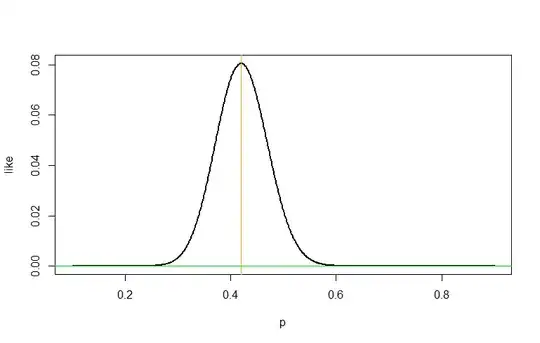
By contrast, if $n = 100,$ then the maximum if much more precisely determined.

x = 42;  n = 100;  p=seq(.1, .9, by = 0.001)
like = dbinom(x, n, p)
plot(p, like, type="l", lwd=2)
abline(h=0, col="green2")

mle = mean(p[like == max(like)])  #'mean' in case of ties with discrete p
mle
[1] 0.42
abline(v = mle, col="orange")

enter image description here

Here he Jeffries interval estimate is $(0.317, 0.508).$

qbeta(c(.025,.975), 41.5, 59.5)
[1] 0.3172977 0.5078283

For the best estimation we need for the curvature of the likelihood curve to be as tight, on average, as possible at the value of the MLE.

BruceET
  • 47,896
  • 2
  • 28
  • 76