Although comments to the question indicate the original problem assumes the $u_t$ have Normal distributions, it is of interest to determine the extent to which this distributional assumption is needed to prove the $x_t$ are not serially dependent.
Let's begin, then, with a clear statement of the problem. It focuses on three variables $(u_{t-1}, u_t, u_{t+1}).$ Suppose they are identically and independently distributed (iid); and that this distribution has zero mean and a finite variance of $\sigma^2.$ (We drop any Normality assumption.) Out of these variables we construct two others, $x_{t+1}=u_{t+1}u_t$ and $x_t = u_tu_{t-1},$ which are products of successive $u$'s. Since $u_t$ is involved in the construction of both of the $x$'s, intuitively those $x$'s should not be independent. But how to prove this?
This is trickier than it might appear, because in simulations with Normally distributed $u$'s, the scatterplot of $(x_t, x_{t+1})$ shows a complete lack of correlation:
Indeed, if we try to demonstrate lack of independence by showing there is nonzero covariance, we will fail (because the $u$'s are independent and have zero mean):
$$\begin{aligned}
\operatorname{Cov}(x_t, x_{t+1}) &= E[x_tx_{t+1}]-E[x_t]E[x_{t+1}]\\
&= E[u_{t-1}u_t\, u_tu_{t+1}] - E[u_{t-1}u_t]E[u_tu_{t+1}]\\
&=E[u_{t-1}]E[u_t^2]E[u_{t+1}] - E[u_{t-1}]E[u_t]\,E[u_t]E[u_{t+1}]\\
&= 0-0 = 0.
\end{aligned}$$
The simplest way I have found to demonstrate lack of independence is to consider the magnitudes of the $x$'s. The logic will be this: if we can show that some function $f$ (in this case, the absolute value) when applied to both $x$'s, produces variables with nonzero covariance, then the $x$'s could not originally have been independent. (A simple proof is at https://stats.stackexchange.com/questions/94872.)
So, let's carry out the preceding calculations using the absolute values. We are permitted to do this because the finite variance of the $u$'s implies the expectations of their absolute values are finite, too (see Prove that $E(X^n)^{1/n}$ is non-decreasing for non-negative random variables). Let this common expectation be $E[|u_t|]=\tau.$ Then
$$\begin{aligned}
\operatorname{Cov}(|x_t|, |x_{t+1}|) &= E[|x_t||x_{t+1}|]-E[|x_t|]E[|x_{t+1}|]\\
&=E\left[|u_{t-1}|\right]E\left[|u_t|^2\right]E\left[|u_{t+1}|\right] - E\left[|u_{t-1}|\right]E\left[|u_t|\right]\,E\left[|u_t|\right]E\left[|u_{t+1}|\right]\\
&= \tau \sigma^2 \tau - \tau^4\\
&= \tau^2(\sigma^2 - \tau^2).
\end{aligned}$$
Unless $\sigma^2=\tau^2$ or $\tau=0,$ this is nonzero and we are done.
Because squaring is a convex function, Jensen's Inequality implies $\tau^2\le\sigma^2$ with equality if and only if $u_t$ is almost surely constant.
The case $\tau=0$ occurs when $|u_t|$ is almost surely constant, whence $u_t$ itself is either $0$ or takes on the values $\pm\sigma$ with equal probability (a scaled Rademacher variable). Both situations can be characterized as scaled Rademacher variables (with scaling factor $0$ in the first case).
That covers all the possibilities. The result is,
When $(u_{t-1}, u_t, u_{t+1})$ are iid with zero mean, $x_t = u_{t-1}u_t$ and $x_{t+1} = u_t u_{t+1}$ are independent if and only if the $u$'s each have a scaled Rademacher distribution.
(The "if" part can be shown with a direct calculation: tabulate the eight possible values of $(u_{t-1}, u_t, u_{t+1}),$ compute the corresponding values of $(x_t, x_{t+1}),$ and verify independence.)
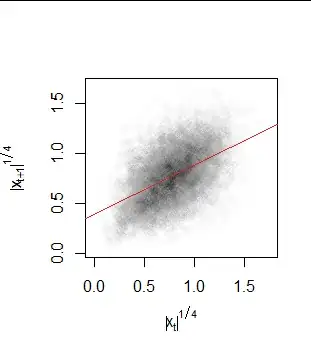
To help the intuition, here is a scatterplot of the absolute values in the preceding figure (shown on fourth-root scales to remove the skewness from the marginal distributions; if you like, the function involved is $f(x) =\sqrt[4]{|x|}$). The red line is the least-squares fit to these fourth roots. The correlation is obviously nonzero.