The mean minimizing the root mean square error is often not the practical situation
It is well known that the mean E(Y |X) minimizes the Root Mean Square Error (RMSE).
You are right, the theoretical mean $E(Y |X) $ minimizes the root mean square error of a prediction (independent of the distribution). So if minimizing the mean square error of a prediction is your goal and you know the theoretical mean, then indeed you do not need to care about the distribution (except whether the mean and variance exist for the distribution).
However, often this theoretical mean is unknown and we use an estimate instead. Or we want to minimize something else than the mean squared error. In those cases you often need to use assumptions about the distribution of the errors in order to determine which estimator to use (to determine which one is optimal).
So a typical situation is
- gathering data from a population
- compute an estimate of the distribution of the population based on the data
- use the estimates directly (e.g. make some decision based on the estimates)
- or use the estimates to make a prediction (in which case the error due to the randomness in the population get's on top of the randomness of the estimates about this population)
The situation that you sketch makes a shortcut to the final point and assumes that we know the population. This is very often not the case. (It can still be a practical case, for instance if we have so much information, a large sample, such that we can estimate the population distribution with high accuracy and the biggest error in the prediction is due to the randomness in the population)
If the predicted value of machine learning method is $E(y | x)$, why bother with different cost functions for $ y | x$?
A machine learning method does not provide $E(y|x)$ it provides an estimate of $E(y|x)$. How good or bad estimators and predictors are will depend on the underlying distribution of the population (from which we can deduce the sample distribution of our estimator and predictor).
Example: Say we wish to estimate the location parameter of a Laplace distributed population (and use that for prediction). In that case the sample median is a better estimator than the sample mean (ie. The distribution of the sample median will be closer to the true parameter than the distribution of the sample mean. The error of the estimate will be smaller).
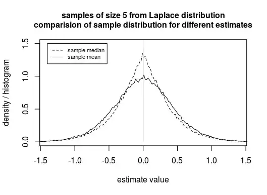
Image: showcase that the sample median can be a better estimator than the sample mean. Note that the distribution is more concentrated around the true location parameter (in this example this is 0).
So based on the assumption that the errors are Laplace distributed we should decide to use the sample median as an estimator and predictor, and not the sample mean.
Difference between cost function used for fitting and cost function used for evaluation.
Another underlying issue is about the differences in cost functions.
The cost function that is used to perform the fitting can be different from the cost function that is the objective.
In the previous example with the Laplace distribution, the objective might be to minimize the expected mean squared error of the estimate/prediction. But, we find the estimate that optimizes this objective by minimising the mean absolute error of the residuals.
A related question is: Could a mismatch between loss functions used for fitting vs. tuning parameter selection be justified? In that question you minimize the (objective) cost function by cross validation, but in the answer it is demonstrated that it is still good to perform the fitting (during training) by means of a cost function that relates to the distribution of the error of the measurements.
quote from the chat
"My question had to do with how to choose one estimator or another one (i.e. one loss function over another one)"
An estimator can be expressed as the argmin of some cost function of the data/sample (e.g. the sample mean minimizes the sum of squared residuals, and the sample median minimizes the sum of absolute residuals).
However, that is a different cost function than the cost function used to describe the performance of an estimator.
So that's why we are bothered with cost functions. Those cost functions allow us to evaluate the performance of an estimator. We can compute/estimate how often an estimator X make a particular error and compare it with how often an estimator Y makes that particular error. And since there are many sizes of errors we make a weighted sum of all possibilities by some cost function.
E.g. the distribution of errors for estimator X and Y might be (a simplistic example)
Error size.                  -2     -1     0      1     2
frequency for estimator X   0.00   0.25   0.50  0.25   0.00
frequency for estimator Y   0.02   0.18   0.60  0.18   0.02
The estimator X has a higher mean absolute error (half the time the error is $\pm1$ and the mean absolut error is 0.5. For the estimator Y it is 0.44).
However in terms of the expected mean squared error the estimator X (with 0.5) is lower than the estimator Y (with expected mean squared error 0.52).
To compute these comparisons you need to be able to know/estimate the sample distribution of the estimators (like in the above example this is done for the Laplace distribution and the sample mean and the sample median) and some cost function to compare those distributions.
(In the case of the Laplace distribution and the sample mean vs sample median, you have that the sample median is stochastically dominant and for any convex cost function the sample median will be better than the sample mean, so you do not always need to know the evaluation cost function in detail. Related question: Estimator that is optimal under all sensible loss (evaluation) functions)
R-code to create the graph
### generate data
set.seed(1)
s <- 100000
n <- 5
x <- matrix(L1pack::rlaplace(s*n,0,1),s)
medians <- apply(x,1,median)
means <- apply(x,1,mean)

### compute frequency histogram
breaks <- seq(floor(min(medians,means)),ceiling(max(medians,means)), 0.02)
hmedians <- hist(medians, breaks = breaks)
hmeans <- hist(means, breaks = breaks)

### plot results
plot(hmedians$mids, hmedians$density, type = "l",
     ylim=c(0,1.5), xlim = c(-1.4,1.4),
     xlab = "estimate value", ylab = "density / histogram",
     lty=2)

lines(hmeans$mids, hmeans$density)
lines(c(0,0),c(0,2),lty=1,col="gray")
title("samples of size 5 from Laplace distribution
comparision of sample distribution for different estimates", cex.main = 1)

legend(-1.4,1.5, c("sample median","sample mean"), lty = c(2,1), cex = 0.7)
