Let's generalize both questions so we don't have to solve them twice:
Let there be $n\ge 0$ bins indexed $1,2,\ldots, n.$ Suppose there are $C\gt 0$ different colors of marbles and $0\le k\le n$ marbles of each color. Distribute each set of $k$ marbles into $k$ distinct bins randomly. Collect all marbles from bin $1,$ then bin $2,$ and so on until you first obtain $m\ge 0$ (and $m\le k$) of at least one color. Let $I$ be the index of the bin you last emptied.
What is the distribution of $I?$ Specifically, what is its 50th percentile?
This abstract rephrasing suggests some useful simplifications:
Each color $c$ determines a simple random sample (without replacement) of the bins. Sorting the bin indexes, we may express this sample as the indexes $1 \le X^{(c)}_1 \lt X^{(c)}_2 \lt \cdots \lt X^{(c)}_k \le n.$
Therefore, $X^{(c)}_m$ (which is the $m^\text{th}$ order statistic of this sample) is the index at which we will have first collected $m$ marbles of color $c.$
Consequently, $I$ is the minimum over all colors of $X^{(c)}_m.$ The specifications of the problem imply these random variables are identically distributed and independent (iid).
That reduces the question to two simpler subproblems. First (dropping the superscript $(c)$), find the distribution of $X_m.$ Second, find the distribution of the minimum of $C$ iid variables.
First subproblem
Let $1\le i\le n$ be a possible value of $X_m.$ Compute the distribution function $F_{m;\,n,k}$ of $X_m$ from its definition,
$$F_{m;\,n,k}(i) = \Pr(X_m \le i) = \Pr(\text{the sample includes at least } m \text{ bins in }\{1,2,\ldots, i\}).$$
Partitioning the event "at least $m$" into the disjoint events "exactly $m,$" "exactly $m+1,$" and so on enables us immediately to express this in terms of Binomial coefficients as
$$F_{m;\,n,k}(i) = \frac{1}{\binom{n}{k}}\sum_{j=m}^k \binom{i}{j}\binom{n-i}{k-j},$$
a hypergeometric tail probability.
Second subproblem
Let $F$ be any distribution on the integers $\{1,2,\ldots, n\}.$ The distribution of the minimum of $C$ iid samples $X_1, \ldots, X_C$ of $F$ is
$$\begin{aligned}
F^{(C)}(i) &= \Pr(\min(X_c)\le i) \\
&= 1 - \Pr(X_1\gt i)\Pr(X_2\gt i)\cdots\Pr(X_C\gt i) \\
&= 1 - (1 - F(i))^C.
\end{aligned}$$
The distribution of $I$
Applying this to the previous result shows
$$\Pr(I \le i) = F^{(C)}_{m;\,n,k}(i) = 1 - (1 - F_{m;\,n,k}(i))^C.$$
Solution to the original problem
The second question asks for the smallest $i$ for which $F^{(100)}_{3;\,99,5}(i) \ge 50\%.$
We may find that by a direct search: the value is $11,$ just barely: $F^{(100)}_{3;\,99,5}(10) = 0.4963\ldots$ while $F^{(100)}_{3;\,99,5}(11) = 0.6059\ldots$ .
Simulation
As a check, I simulated 10,000 independent repetitions of the process described in the second question (which, because it distributes balls into bins a million times, takes a few seconds).
Here are plots of the empirical distribution of $X_3$ (in black) compared to its probability function $f$ and distribution function $F$ (in red):
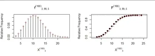
The answer to question #2, by the way, is found by inspecting the red points in the right hand plot (showing the distribution of $X^{(C)}_m$) to find the leftmost one at a height of $0.5$ or greater. Because the height at $10$ is almost exactly $0.5,$ it's necessary to look at its value (slightly less than $0.5$) to discover the correct answer must be $11.$
The agreement between simulation and theory is excellent, as confirmed by a $\chi^2$ test (df = 21, p = 0.57) as well as this "rootogram" comparing the empirical frequencies by plotting the difference in their roots against their expected square root:
All residuals (but one, near the left) are small and display no trend. Repeated simulations confirm there is no systematic problem.
Code
This R code implements the formula for $F$ (efficiently) and generates the simulation and figures. You may use it to study the first question.
#
# Sample randomly from a process.
#
rcolor <- function(N, n, k, m, C=1) {
  replicate(N,
            min(replicate(C, {
              x <- sample.int(n, k)
              x[order(x)[m]]
            })))
}
#
# Compute the distribution function.
#
pcolor <- function(i, n, C, k, m) {
  i <- pmin(n-1, i+1)
  1 - exp(C * phyper(m-1, i, n-i, k, log.p=TRUE))
}
#
# Create the simulation.
#
n <- 99
m <- 3
k <- 5
C <- 100
set.seed(17)
x <- rcolor(1e4, n, k, m, C)
#
# Create figure 1.
#
y <- tabulate(x, n)
y <- y / sum(y)
p <- diff(P <- pcolor(0:n, n, C, k, m))
i <- seq(min(x), max(x)) # Limits plots to the observed values

par(mfrow=c(1,2))
plot(i, y[i], type="h", xlab=bquote({X^{(.(C))}}[.(m)]), ylab="Relative Frequency",
     main=bquote({f^{(.(C))}}[list(.(m), .(n), .(k))]))
points(i, p[i-1], col="Red", cex=1)

plot(ecdf(x), xlab=bquote({X^{(.(C))}}[.(m)]), ylab="Relative Frequency",
     main=bquote({F^{(.(C))}}[list(.(m), .(n), .(k))]))
points(i, P[i], col="Red", cex=1.25)
par(mfrow=c(1,1))
#
# Create figure 2.
#
x.tot <- tabulate(x, max(i))[i]
P[max(i)] <- 1
prob <- diff(P[c(min(i)-1, i)])  # The probability function `f`.
plot(sqrt(prob * length(x)), sqrt(x.tot) - sqrt(prob * length(x)), type="h",
     main="Rootogram",
     ylab="Residual", xlab=expression(sqrt(expected * phantom(0) * frequency)))
abline(h=0, col="Gray", lwd=1)
#
# Formally compare the simulation to the theory.
# (Ignore the warning: the few small-expectation bins don't harm the chi-squared
# approximation used to compute the p-value.)
#
chisq.test(x.tot, p=prob)

