Why is the coverage of this lme4 confidence interval less than 95%?

Question

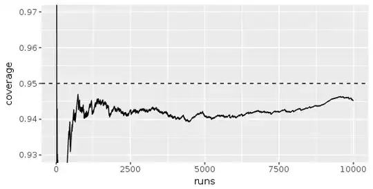
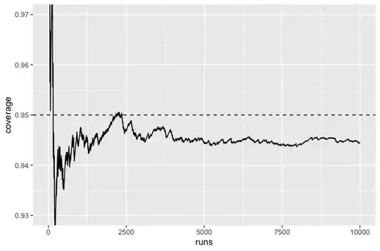
I have data that can be described using the model $y_{i j} = \alpha_i + \epsilon_{i j}$, where $\alpha_i \sim \text{N}(\mu_{\alpha}, \sigma_{\alpha}^2)$ and $\epsilon_{i j} \sim \text{N}(0, \sigma_{\epsilon}^2)$. There are 768 observations in 48 groups of 16 observations each, so $i = 1, \ldots, 48$ and $j = 1, \ldots, 16$. I want to calculate a 95% confidence interval for $\mu_{\alpha}$. I decided to try fitting the model $\tt{y \sim (1 \ | \ group)}$ to the data using the lme4 package and computing a confidence interval using the package's $\tt{confint()}$ function. I created a simulation to check the coverage of the confidence interval; the code is below. It seems like the coverage is around 94.5% instead of 95%. Is there a flaw in my simulation, or is this result to be expected?

# Load packages -----------------------------------------------------------

library(lme4)
library(tidyverse)

# Define functions --------------------------------------------------------

make_dataset <- function(groups, group_size,
                         mu_alpha, sigma_alpha, sigma_epsilon) {
  replicate(
    groups,
    {
      group_mean <- rnorm(1, mean = mu_alpha, sd = sigma_alpha)
      errors <- rnorm(group_size, sd = sigma_epsilon)
      tibble(y = group_mean + errors)
    },
    simplify = FALSE
  ) %>%
    bind_rows(.id = "group") %>%
    mutate(group = as_factor(group))
}

check_conf_int <- function(dataset, mu_alpha) {
  mod <- lmer(y ~ (1 | group), dataset)
  conf_int <- confint(mod, "(Intercept)")
  between(mu_alpha, conf_int[, "2.5 %"], conf_int[, "97.5 %"])
}

# Set simulation parameters -----------------------------------------------

groups <- 48
group_size <- 16
mu_alpha <- 0
sigma_alpha <- 1
sigma_epsilon <- 0.25
runs <- 10000

# Make datasets -----------------------------------------------------------

set.seed(1)

# Takes 5 minutes
datasets <- replicate(
  runs,
  make_dataset(groups, group_size, mu_alpha, sigma_alpha, sigma_epsilon),
  simplify = FALSE
)

# Run simulation ---------------------------------------------------------

# Takes 30 minutes
results <- map_lgl(datasets, check_conf_int, mu_alpha = mu_alpha)

tibble(
  runs = seq_len(runs),
  coverage = cummean(results)
) %>%
  ggplot(aes(runs, coverage)) +
  geom_line() +
  geom_hline(linetype = "dashed", yintercept = 0.95) +
  coord_cartesian(ylim = c(0.93, 0.97))

Below is the plot produced by the last code chunk:

Below is the output of $\tt{sessionInfo()}$:

R version 4.0.0 (2020-04-24)
Platform: x86_64-apple-darwin17.0 (64-bit)
Running under: macOS Catalina 10.15.6

Matrix products: default
BLAS:   /System/Library/Frameworks/Accelerate.framework/Versions/A/Frameworks/vecLib.framework/Versions/A/libBLAS.dylib
LAPACK: /Library/Frameworks/R.framework/Versions/4.0/Resources/lib/libRlapack.dylib

locale:
[1] en_US.UTF-8/en_US.UTF-8/en_US.UTF-8/C/en_US.UTF-8/en_US.UTF-8

attached base packages:
[1] stats     graphics  grDevices utils     datasets  methods   base     

other attached packages:
 [1] forcats_0.5.0   stringr_1.4.0   dplyr_0.8.5     purrr_0.3.4     readr_1.3.1    
 [6] tidyr_1.0.3     tibble_3.0.1    ggplot2_3.3.0   tidyverse_1.3.0 lme4_1.1-23    
[11] Matrix_1.2-18  

loaded via a namespace (and not attached):
 [1] statmod_1.4.34   tidyselect_1.1.0 xfun_0.13        splines_4.0.0   
 [5] haven_2.2.0      lattice_0.20-41  colorspace_1.4-1 vctrs_0.3.0     
 [9] generics_0.0.2   htmltools_0.4.0  yaml_2.2.1       rlang_0.4.6     
[13] nloptr_1.2.2.1   pillar_1.4.4     withr_2.2.0      glue_1.4.0      
[17] DBI_1.1.0        dbplyr_1.4.3     modelr_0.1.7     readxl_1.3.1    
[21] lifecycle_0.2.0  cellranger_1.1.0 munsell_0.5.0    gtable_0.3.0    
[25] rvest_0.3.5      evaluate_0.14    labeling_0.3     knitr_1.28      
[29] fansi_0.4.1      broom_0.5.6      Rcpp_1.0.4.6     backports_1.1.6 
[33] scales_1.1.1     jsonlite_1.6.1   farver_2.0.3     fs_1.4.1        
[37] hms_0.5.3        packrat_0.5.0    digest_0.6.25    stringi_1.4.6   
[41] grid_4.0.0       cli_2.0.2        tools_4.0.0      magrittr_1.5    
[45] crayon_1.3.4     pkgconfig_2.0.3  MASS_7.3-51.6    ellipsis_0.3.0  
[49] xml2_1.3.2       reprex_0.3.0     lubridate_1.7.8  assertthat_0.2.1
[53] minqa_1.2.4      rmarkdown_2.1    httr_1.4.1       rstudioapi_0.11 
[57] R6_2.4.1         boot_1.3-25      nlme_3.1-147     compiler_4.0.0

Updates

Below is the plot I get if I increase groups to 480:

This is the plot I get when I change group_size to 160:

Answer 1

The issue here is that the mean coverage will only converge to 0.95 as the number of groups becomes large. When the number of groups is "low" then I believe you will find on average less than 95% coverage. 48 is neither particularly high or low. However, with a typical 94.5% coverage with your parameters, I don't think this is a big problem in this case.

Also, the pattern you see in your plot are only relevant for the particular seed you set.

To see this, we can run some more simulations. Note that I have modified your code to make it run in parallel on as many local cores as you have available. This type of simulation is particularly suited to parallelisation. Doing this reduced the run time on my machine from over 28 minutes to under 6 minutes with 48 groups and 16 subjects per group :)

I have also added a progress bar for the main simulation so you are not waiting around wondering how long it's going to take:

library(lme4)
library(tidyverse)
library(parallel)
library(purrr)
library(furrr)

check_conf_int <- function(dataset, mu_alpha) {
  mod <- lmer(y ~ (1 | group), dataset)
  conf_int <- confint(mod, "(Intercept)", quiet = TRUE)
  between(mu_alpha, conf_int[, "2.5 %"], conf_int[, "97.5 %"])
}

runs <- 10000
mu_alpha <- 0  # note : also needs to be set in the cluster

for (seed in 1:10) {

  set.seed(seed)

  cl <- makeCluster(detectCores()-1)  

  # send data, packages and function to the cores
  clusterEvalQ(cl,
             {
              library(magrittr);library(dplyr)
              groups <- 96
              group_size <- 16
              mu_alpha <- 0
              sigma_alpha <- 1
              sigma_epsilon <- 0.25
 
              make_dataset <- function(groups, group_size,
                                      mu_alpha, sigma_alpha, sigma_epsilon) {
                  replicate(
                  groups,
                  {
                   group_mean <- rnorm(1, mean = mu_alpha, sd = sigma_alpha)
                   errors <- rnorm(group_size, sd = sigma_epsilon)
                   tibble(y = group_mean + errors)
                  },
                  simplify = FALSE
                  ) %>%
                   bind_rows(.id = "group") %>%
                  mutate(group = as.factor(group))
               }
             }
  ) 

  # create a parallel version of replicate
  parReplicate <- function(cl, n, expr, simplify = TRUE, USE.NAMES = TRUE) {
  parSapply(cl, integer(n), function(i, ex) eval(ex, envir = .GlobalEnv),
            substitute(expr), simplify = simplify, USE.NAMES = USE.NAMES)
  }

  datasets <- parReplicate(
    cl,
    runs,
    make_dataset(groups, group_size, mu_alpha, sigma_alpha, sigma_epsilon),
    simplify = FALSE
  )

  stopCluster(cl)

  future::plan(multiprocess)
  results <- future_map(datasets, check_conf_int, mu_alpha = mu_alpha, .progress = TRUE)

  p <- (tibble(
    runs = seq_len(runs),
    coverage = cummean(results)
  ) %>%
    ggplot(aes(runs, coverage)) +
    geom_line() +
    geom_hline(linetype = "dashed", yintercept = 0.95) +
    coord_cartesian(ylim = c(0.93, 0.97)) 
 )

  print(p)
}

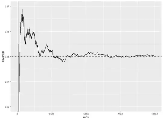
The following two plots are for 96 groups:

As you can see, these show much better coverage. And finally, one with 200 groups.