Distribution of the inner product between a noise-free and a noisy signal

Question

I am working on a problem where we have a noisy measured signal, which is stored as an $N$-dimensional vector $\mathbf{Y},$ and a set of $n_s$ simulated noise-free signals $\{\mathbf{X}_i\}_{i=1}^{n_s}.$ Our goal is to identify which of the simulated signals $\mathbf{X}_i$ best matches $\mathbf{Y},$ which we define as the simulated signal with the highest normalized dot product $\mathbf{Y}$:

$$\rho_i = \frac{\mathbf{Y} \cdot \mathbf{X}_i}{\|\mathbf{Y}\| \|\mathbf{X}\|}$$

where $\rho_i$ is sometimes called the cosine similarity score, and is constrained to have values between $-1$ and $1.$ The question I want to ask is: if each element of $\mathbf{Y}$ has a Gaussian distribution with standard deviation $\sigma$, then is there an analytical expression for the distribution of $\rho_i?$ Specifically, I would like to be able to get expressions for the mean and variance of $\rho_i.$

To simplify the investigation, I am considering a situation where we have a single noise free signal $\mathbf{X}$, and a noise-corrupted version of this: $\mathbf{Y}=\mathbf{X} + \boldsymbol{\eta}$, where each element of $\boldsymbol{\eta}$, $\eta_j \sim \mathcal{N}(0,\sigma)$ (all elements of $\boldsymbol{\eta}$ have the same standard deviation). Clearly the un-normalized dot product $\mathbf{Y} \cdot \mathbf{X}$ should follow a normal distribution, but as soon as I start including the normalization terms it becomes much more complicated, and I am really not sure how to proceed.

I have looked to see if anybody has posted any similar questions, and this was the closest I could find. However, while this question also concerns the distribution of the cosine similarity score, they appear to consider a rather special case where $\mathbf{X}$ has only one non-zero element, and furthermore it appears that the question was never completely answered.

Numerical simulations

In order to empirically check what the PDFs should look like, I have done a computer simulation where I take a noise-free signal and generate $10,\!000$ noise realizations of that signal (by adding Gaussian noise) and look at the histograms of the normalized dot product values between each noisy signal and the noiseless signal. In the histogram below I repeated this for three different noise levels. As one might expect, at higher noise levels the expected value of $\rho$ is reduced, while the variance increases. The distributions do look somewhat symmetrical, so it may be possible to approximate them as Gaussian under certain circumstances.

$10,\!000$ noise realizations and computed the normalized dot product between each noisy signal and the noise free signal" />

Answer 1

EDIT: I've added some details to confirm that also this approach provides an accurate estimate of a transformed cosine value, although the answer by @Sextus Empiricus is much more elegant and works better for the specific case of $\mathbf{Y}=\mathbf{X}+\mathbf{\eta}$. (my +1 goes to that answer).

My answer follows pretty much the answer you cited .

This is what I have been able to determine from the simple case scenario of a normally distributed $\mathbf{Y}=(y_1, y_2, \ldots, y_N)$, with $y_i \sim \mathcal{N}(\mu_{Y,i}, \sigma_\eta^2)$:

$$ \mathbf{Y}=\mathbf{\mu_Y}+\mathbf{\eta}\\ \mathbf{\eta} \sim \mathcal{N}(\mathbf{0},\sigma_\eta^2 \mathbf{I}) $$

In this case, the cosine similarity is:

$$ \rho=\frac{\sum_{i=1}^N x_i y_i}{\sqrt{\sum_{k=1}^N x_k^2}\sqrt{\sum_{k=1}^N y_k^2}}= \frac{1}{\sqrt{\sum_{k=1}^N x_k^2}} \times \frac{\sum_{i=1}^N x_i y_i}{\sqrt{\sum_{k=1}^N y_k^2}}=\\ \frac{1}{\sqrt{\sum_{k=1}^N x_k^2}} \times \frac{\sum_{i=1}^N x_i y_i}{\sigma_\eta\sqrt{\sum_{k=1}^N \frac{y_k^2}{\sigma_\eta^2}}}=\\ \frac{1}{||\mathbf{X}||} \times \sum_{i=1}^N x_i \frac{Z_i^{1/2}}{W^{1/2}} $$

where

$$ Z_i=\frac{y_i^2}{\sigma_\eta^2}\\ W=\sum_{i=1}^N \frac{y_i^2}{\sigma_\eta^2}=\sum_{i=1}^N Z_i $$

$W$ is non-central $\chi^2$-distributed with $df=N$ and non-centrality parameter $\sum_{k=1}^N \frac{\mu_{Y,i}^2}{\sigma_\eta^2}$. $Z_i$ is a non central $\chi^2$-distributed with $df=1$ and non-centrality parameter $\frac{\mu_{Y,i}^2}{\sigma_\eta^2}$.

Following the procedure suggested in https://stats.stackexchange.com/a/93741/289381, we can calculate the reciprocal:

$$ \frac{1}{||\mathbf{x}||} \times \sum_{i=1}^N x_i \frac{1}{\left(\sum_{k=1}^N \frac{Z_k}{Z_i}\right)^{1/2}} = \frac{1}{||\mathbf{x}||} \times \sum_{i=1}^N x_i \frac{1}{\left(1+\sum_{k \neq i} \frac{Z_k}{Z_i} \right)^{1/2}} $$

where $\frac{Z_k}{Z_i}$ is a doubly non-central $F$-distributed random variable.

EDIT: $\mathbf{Y}=\mathbf{X}+\mathbf{\eta}$ case:

Using the spherical symmetry, as done by @Sextus Empiricus:

$$ \mathbf{X} \equiv (l, 0, \ldots, 0)\\ \mathbf{Y} \equiv \mathbf{X} + \mathbf{\eta} = (l+\eta_1, \eta_2 \ldots, \eta_N) \sim \mathcal{N}(\mathbf{X}, \sigma_\eta^2 \mathbf{I})\\ \mathbf{\eta} \sim \mathcal{N}(\mathbf{0}, \sigma_\eta^2 \mathbf{I}) $$

In this case, the cosine $\rho$ is

$$ \rho=\frac{\mathbf{X} \cdot \mathbf{Y}}{\lVert \mathbf{X}\rVert \lvert \mathbf{Y} \rVert} = \\ \frac{\sum_{i=1}^N x_i y_i}{(\sum_{i=1}^N x_i^2)^{1/2} (\sum_{i=1}^N y_i^2)^{1/2}}= \frac{1}{l}\frac{l^2 + l\eta_1}{(\sum_{k=1}^N y_i^2)^{1/2}}=\frac{l + \eta_1}{(\sum_{k=1}^N y_i^2)^{1/2}} $$

where the numerator is Normally distributed

$$ l + \eta_1 \sim \mathcal{N}(l, \sigma_\eta^2) $$

We can use the same approach for calculating $1/\rho^2$:

$$ \frac{1}{\rho^2} = 1 + (n-1) \frac{\sum_{i=2}^N \eta_i^2/\sigma_\eta^2}{((l+\eta_1)^2/\sigma_\eta^2)} $$

where $\frac{\sum_{i=2}^N \eta_i^2/\sigma_\eta^2}{((l+\eta_1)^2/\sigma_\eta^2)}$ follows a doubly non-central $F$ distribution with $df_1=N-1$, $df_2=1$ and non-centrality parameters $\lambda_1=0$, $\lambda_2=l^2/\sigma_\eta^2$.

library(sadists)

l = 10
sig = 2
n = 10

set.seed(42)

rho <- numeric(1e4)
for (i in 1:1e4) {
  eta <- rnorm(n, mean = 0, sd = sig) 
  X   <- c(l,rep(0,n-1))
  Y   <- X + eta
  rho[i] <- X %*% Y / sqrt((X %*% X) * (Y %*% Y))
}

yy_dnf <- rdnf(n=1e4, df1=n-1, df2=1, ncp1=0, ncp2=l^2/sig^2)
rrho_2 <- sqrt(1 + (n-1) * yy_dnf)

dd <- density(1/rrho_2)
hist(rho, breaks=seq(min(rho), 1, 1e-2), freq=0)
lines(dd$x, dd$y)

^{Created on 2020-07-27 by the reprex package (v0.3.0)}

Answer 2

In short

The simplified case, with spherically symmetric $\boldsymbol{\eta}$ (that is i.i.d $\eta_j \sim \mathcal{N}(0,\sigma)$), can be related to a transformed non-central t-distribution.

We have:

$$ \sqrt{n-1} \frac{\rho}{\sqrt{1-\rho^2}} \sim T_{\nu = n-1, ncp = l/\sigma} $$

where $l$ is the length of the vector $\mathbf{X}$.

Geometric view of problem, and rotation

We can view the problem by considering the radial and transverse components of the distance of the vector $Y$. These transverse and radial components are defined with respect to the vector $X$.

This means that the direction of $\mathbf{X}$ is not really important, because we consider the situation relative to $\mathbf{X}$

This view is easier when we rotate the vector $\mathbf{X}$ such that it is aligned allong one single axis. For instance, in the code below we generate/simulate samples with the vector $\mathbf{X}$ having only the first component non zero, $\lbrace l,0,0,\dots,0,0 \rbrace$. We can do this without loss of generality.

In the case that $\boldsymbol{\eta}$ has i.i.d. $\eta_j \sim \mathcal{N}(0,\sigma)$, then the distribution will be spherically symmetric. This means that after the rotation the distribution of the rotated $\boldsymbol{\eta}$ can still be considered to have i.i.d. components.

See the image below where we rotate the situation (to align the vector $\mathbf{X}$ to a basis vector). On the left we see the situation for the complex situation (not all $\eta_j$ identical but with different variance) and on the right we see the situation for the simplified case.

Now we can attack the problem by focussing on the angle, $\phi$, between $\mathbf{X}$ and $\mathbf{Y}$. The actual direction of $\mathbf{X}$ does not matter, and we can parameterize the distribution by only the length of $\mathbf{X}$, say $l$.

The angle $\phi$ can be described by its cotangent, the ratio of the the radial and transverse parts of the vector $Y$ relative to $X$.

Note that, with the rotated vector $\mathbf{X} \sim \lbrace l, 0, 0, \dots, 0, 0 \rbrace$ the components of $\mathbf{Y}$ are easier to express

$$Y_i \sim \begin{cases} N(l,\sigma)\quad \text{if} \quad i=1 \\ N(0,\sigma)\quad \text{if} \quad i\neq 1\end{cases}$$

and we can easily express the radial part, $Y_1$, and the transverse part, $\lbrace Y_2,Y_3, \dots, Y_{n-1}, Y_{n} \rbrace$. And the lengths will be distributed as:

• The length of the radial part is a Gausian distributed variable

• The length of the transverse part is a scaled $\chi_{n-1}$ distributed variable.

  (The image is in 2D for simplicity of plotting, but you should imagine this in a multidimensional way. The length of the transverse part is a sum of $n-1$ components. A similar construction is shown here where a 3D visualization of the angle is shown)

This ratio of the radial and transverse part, multiplied with $\sqrt{\nu}$, lets call it $T_{l/\sigma,nu}$, has a t-distribution with non-centrality parameter $l/\sigma$ and degrees of freedom $\nu = n-1$ (were $n$ is the dimension of your vectors).

note: this t-distribution occurs because the radial part and transverse part are independently distributed in the simplified problem. In the generalized problem this will not work (although the limit, large $n$, may still be useful when we appropriately adapt the scaling factor). See this in the first image on the left, where after rotation the distribution of $Y$ shows a correlation between transverse and radial part, and also the transverse part is not anymore $\sim \chi_{n-1}$, because the individual component may have different variance.

The transformation between $T_{l/\sigma}$, which is the cotangent of the angle (multiplied with $\sqrt{\nu}$), and your dot product $\rho$, which is the cosine of the angle is:

$$\rho = \frac{T_{l/\sigma}}{\sqrt{\nu+T_{l/\sigma}^2}}$$

$$T_{l/\sigma} = \sqrt{\nu} \frac{\rho}{\sqrt{1-\rho^2}}$$

If $f(t,\nu,l/\sigma)$ is the non-central distribution (which is a bit awkward to write down, so I just write it as $f$), then the distribution $g(\rho)$ for the dotproduct is

$$g(\rho) = f\left(\sqrt{\nu} \frac{\rho}{\sqrt{1-\rho^2}},\nu,l/\sigma\right) \frac{\sqrt{\nu}}{(1-\rho^2)^{3/2}} $$

That distribution is a bit difficult to write down. It might be easier to work with a transformed correlation coefficient

$$ \sqrt{n-1} \frac{\rho}{\sqrt{1-\rho^2}} \sim T_{\nu = n-1, ncp = l/\sigma} $$

For large $n$ this will approximate a normal distribution.

---

Simulation

l = 10
sig = 2
n = 10

set.seed(1)

simulate = function(l, sig , n) {
    eta <- rnorm(n, mean = 0, sd = sig)  
    X   <- c(l,rep(0,n-1))
    Y   <- X + eta
    out1 <- (Y %*% X)/sqrt(X %*% X)/sqrt(Y %*% Y)  # this one is rho
    out2 <- sqrt(n-1)*Y[1]/sqrt(sum(Y[-1]^2))                # this is related non central t-distributed
    c(out1,out2) 
}

rhoT <- replicate(10^4, simulate(l,sig,n))
rho <- rhoT[1,]
t <-   rhoT[2,]

# t-distribution
hist(t,breaks = 20, freq = 0)
ts <- seq(min(t),max(t),0.01)
lines(ts,dt(ts,n-1,ncp=l/sig))

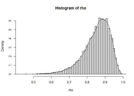
# distribution of rho which is transformed t
hist(rho, freq = 0, breaks = seq(0,1,0.01))

rhos <- seq(-0.999,0.999,0.001)
lines(rhos,dt(x = rhos*sqrt(n-1)/sqrt(1-rhos^2),
              df = n-1,
              ncp = l/sig)*sqrt(n-1)/(1-rhos^2)^1.5)

---

Non simplified problem

In this case the $\boldsymbol{\eta}$ is not symmetric and the view of the ratio of a horizontal and vertical part (relating to a t-distribution) does not work so well. The two parts may be correlated and also the vertical part is not anymore chi-distributed but will be related to a sum of the square of correlated normal distributed variables with different variance.

However, I guess that for large dimension $n$ we may expect that the transformed variable will approach again a normal distribution (but the scale factor depending on the degrees of freedom $\nu=n-1$ may need to be adapted).

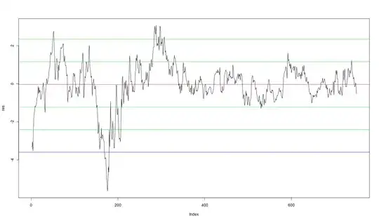
Below is a simulation that demonstrates this:

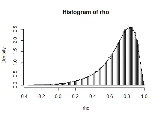
These simulations indicate that a t-distribution still fits well, but we need to use a different effective scaling, different non-central parameter and different degrees of freedom. In the image the curve is drawn based on fitting those parameters. I believe that it will be difficult to find exact expressions for these parameters, but I guess that it is safe to say that it will still be approximately a transformed non-central t-distribution.

#### defining parameters
### 
set.seed(1)
n = 10
l = 10

sigspread = 3  ### the higher this number the smaller the spread of the different sigma
sig = 2*rchisq(n,sigspread)/sigspread

X <- rnorm(n,1,1)
### make the vector X equal to size/length "l"
lX <- sqrt(sum(X^2))
X <- X*(l/lX)



### function to simulate a sample and compute the different statistics
### rho, the radial and transverse parts and the cotangent which is related to rho
simulate = function(l, sig , n) {
  eta <- rnorm(n, mean = 0, sd = sig)  
  Y   <- X + eta
  out1 <- (Y %*% X)/sqrt(X %*% X)/sqrt(Y %*% Y)  # this one is rho
  radial <- (Y %*% X)/sqrt(X %*% X)
  transverse <- sqrt(sum(Y^2)-radial^2)
  out2 <- sqrt(n-1)*radial/transverse            # this is related to rho and non central t-distributed
  c(out1,out2,radial,transverse) 
}

### simulate a sample to make the histogram
rhoT <- replicate(10^5, simulate(l,sig,n))

### the simulated values
rho <- rhoT[1,]
t <-   rhoT[2,]
radial     <- rhoT[3,]
transverse <- rhoT[4,]

###  fitting of the transformed variable
hfit <- hist(rho/(1-rho^2)^0.5, breaks = 100, freq = 0)
yfit <- hfit$density
xfit <- hfit$mids

### fitting
mod <- nls(yfit ~ dt(xfit*scale, nu, ncp)*scale, 
           start = list(nu = n-1, ncp = l/sqrt(mean(sig^2)), scale = sqrt(n-1)),
           lower = c(1,0,0.1),
           upper = c(n*2, l/sqrt(mean(sig^2))*2,10), algorithm = "port")
coef <- coefficients(mod)

### curve which is naive initial guess
lines(xfit, dt(xfit*sqrt(n-1), 
               df = n-1,  
               ncp = l/sqrt(mean(sig^2))
)*sqrt(n-1), col = 2 )
### curve which is fitted line
lines(xfit, dt(xfit*coef[3], df = coef[1],  ncp = coef[2])*coef[3], col = 4 )

### plotting rho with fitted value
h <- hist(rho, freq = 0, breaks = 100)
rhos <- seq(-0.999,0.999,0.001)
lines(rhos,dt(x = rhos/(1-rhos^2)^0.5*coef[3],
              df = coef[1],
              ncp = coef[2])/(1-rhos^2)^1.5*coef[3])


### initial estimates
c(nu=(n-1),
     ncp = l/sqrt(mean(sig^2)),
     scale = sqrt(n-1))
### fitted values
coef