It is said that “the finite population correction factor is used when you sample without replacement from more than 5% of a finite population. It’s needed because under these circumstances, the central limit theorem doesn’t hold true and the standard error of the estimate will be too big.” This is weird cause intuitively the bigger the sample size is, the more central limit theorem must be true and the amount of standard error must be decreased. If having a big sample have these problems so why we bother ourselves to have a big sample? Intuitively if our sample is bigger, our problems must be less!! What is the explanation?
- 63,378
- 26
- 142
- 467
- 93
- 5
-
1Welcome to CV, Zhaleh. – Alexis Jul 24 '20 at 18:25
-
1In sampling _with_ replacement, each draw is independent of the previousone. // In sampling _without replacement,_ what's left of the population depends on what members of the population were sampled previously. // If less than 5% or 10% of the population is sampled, then the impact of a few missing members of the population is not so large for subsequent sampling. So, in taking a tiny sample from a huge population, one can ignore the difference between sampling with and without replacement. In terms of dist'ns, one uses binomal for sampling with repl. and hypergeometric for sampling without. – BruceET Jul 24 '20 at 21:14
-
1Your source is not being helpful to you there. The finite population correction factor has *nothing whatever* to do with the CLT; it has to do with the ratio of the sd of the hypergeometric to the sd of the binomial and is a small sample result. (It sounds like you're also perhaps being somewhat misled about the CLT; you might need a better source for that) – Glen_b Jul 25 '20 at 06:48
-
Also see https://stats.stackexchange.com/questions/346575/what-is-the-formula-of-the-finite-population-correction-factor/346663#346663 or https://stats.stackexchange.com/questions/80162/standard-error-of-proportion-that-takes-into-account-population-size/80195#80195 – Glen_b Jul 25 '20 at 06:55
1 Answers
Comment continued, to show graphs of some specific distributions.
Scenario 1. Urn with 5 red chips and 10 blue ones. Sample 4 chips at random with replacement. Then the number $X$ of red chips drawn is $\mathsf{Binom}(n=4, p=1/3),$ so that $E(X) = np = 4/3; Var(X) = np(1-p) = 4(1/3)(2/3) = 8/9 = 0.8889.$
x=0:4; pdf.b = dbinom(x, 4, 1/3)
mean = sum(x*pdf.b); mean
[1] 1.333333
var = sum((x-mean)^2*pdf.b); var
[1] 0.8888889
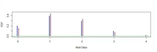
Scenario 2. Same as in Scenario 1, except that the number $Y$ of red chips drawn is a nypergeometric distribution in which $P(X = k) = \frac{{5\choose k}{10\choose 4-k}}{{15 \choose 4}},$ for $k = 0,1,2,3,4.$ Thus, $E(Y) = 4(5/15) = 4/3;$ $Var(Y) = 4(5/15)(10/15)(11/14) = 88/126 = 0.6984.$ The smaller variance reflects the decreasing choices available in later draws as the number of remaining chips gets depleated.
y=0:4; pdf.h = dhyper(y, 5,10, 4)
mean = sum(x*pdf.h); mean
[1] 1.333333
mean = sum(y*pdf.b); mean
[1] 1.333333
var = sum((y-mean)^2*pdf.h); var
[1] 0.6984127
The following bar chart of the two distributions, binomial (blue) and hypergeometric (maroon) illustrates the difference between them.
plot((0:4)-.02, pdf.b, type="h", lwd=3, ylim=c(0,.45), col="blue",
     ylab="PDF", xlab="Red Chips", main="")
 points((0:4)+.02, pdf.h, type="h", lwd=3, col="maroon")
 abline(h=0, col="green2")
Scenario 3. Same as Scenario 2, except now there are 500 red chips and 1000 blue ones. Now let $W$ be the number of red chips drawn without replacement in four draws from the urn. One can show that $E(W) = 4/3 = 1.3333; Var(W) = 0.8871.$ Now the variance is almost the same as for the binomial distribution.
W=0:4; pdf.w = dhyper(y, 500,1000, 4)
mean = sum(w*pdf.w); mean
[1] 1.333333
var = sum((w-mean)^2*pdf.w); var
[1] 0.8871099
Furthermore, the distributions of $W$ and $X$ are nearly the same. (In the table, ignore
row numbers in [ ]s.)
round(cbind(Red = 0:4, pdf.b, pdf.w, pdf.h), 3)
     Red pdf.b pdf.w pdf.h
[1,]   0 0.198 0.197 0.154
[2,]   1 0.395 0.395 0.440
[3,]   2 0.296 0.297 0.330
[4,]   3 0.099 0.099 0.073
[5,]   4 0.012 0.012 0.004
Because the resolution of the bar chart is not much better than two decimal places, it hardly shows any difference at all between the binomial distribution and the hypergeometric distribution with a 'population' of 1500 chips (2nd column in the table just above).
plot((0:4)-.02, pdf.b, type="h", lwd=3, ylim=c(0,.45), col="blue",
      ylab="PDF", xlab="Red Chips", main="")
 points((0:4)+.02, pdf.w, type="h", lwd=3, col="maroon")
 abline(h=0, col="green2")
- 47,896
- 2
- 28
- 76

