5

This is a very basic question about Bayesian inference. I'm not grasping one or more fundamental concepts.

Let's say I have two observed outcomes, X and Y. I want to infer the probabilities (px and py, respectively) of each occurring given X and Y. I do not know N, the total number of trials. I'm assuming that X and Y are binomially distributed. How do I calculate the likelihood without N?

What I ultimately want is to show the bivariate posterior distribution of px and py via MCMC. I do not care about estimating N--I just want to show the chain in the plane of px and py. No convergence necessary.


Clarification: X and Y are drawn from the same N: X ~Binom(N, px) and Y ~Binom(N, py). We have no other information about px or py, although I'll use a beta prior to start. Also assume that X and Y are independent.

neophyte
  • 145
  • 8
  • Are X and Y both drawn from the same distibution $Bin(N, p)$? And do we have any information about $p$? – Cam.Davidson.Pilon Jan 07 '13 at 21:30
  • Good questions! Revised post to clarify. – neophyte Jan 07 '13 at 21:32
  • And are you familiar with Python? – Cam.Davidson.Pilon Jan 07 '13 at 21:37
  • Not Python, but C++, Java, Javascript, etc. I am going to use Javascript for this. It might be best to use pseudocode here. – neophyte Jan 07 '13 at 21:37
  • It seems to me like the problem is under-determined. You're trying to guess 3 unknowns (px, py, and N) from 2 data points, with no additional information. I don't think there's any way around that. – David J. Harris Jan 07 '13 at 21:38
  • No such thing as undetermined in Bayesian analysis, we can only be certain our priors will be more influential. – Cam.Davidson.Pilon Jan 07 '13 at 21:40
  • @Cam.Davidson.Pilon Sure, but in this case, the likelihood surface will be almost entirely flat and the prior will dominate almost entirely. – David J. Harris Jan 07 '13 at 21:41
  • I can see how it's underdetermined with respect to _px_ and _py_ separately, but I'm really going after _px_ / _py_, which should produce a banana plot. (This is, ironically, for a MCMC tutorial, and I've conceptually lost the thread of how to get this to work. Users will have the option of switching between beta and uniform priors.) – neophyte Jan 07 '13 at 21:42
  • Actually, I take it back: the likelihood will only be flat for large N. There's a *lot* of curvature near N == max(X, Y). I wouldn't trust inferences near that value much, though... – David J. Harris Jan 07 '13 at 21:54

1 Answers1

7

Model and Pseudocode

So I did some analysis in Python, though I used the pyMC library which hides all the MCMC mathy stuff. I'll show you how I modeled it in semi-pseudocode, and the results.

I set my observed data as $X=5, Y=10$.

X = 5
Y = 10

I assumed that $N$ has a Poisson prior, with the Poisson's rate a $EXP(1)$. This is a pretty fair prior. Though I could have chosen some uniform distribution on some interval:

rate = Exponential( mu = 1 )
N = Poisson( rate = rate)

You mention beta priors on $pX$ and $pY$, so I coded:

pX = Beta(1,1) #equivalent to a uniform
pY = Beta(1,1)

And I combine it all:

observed = Binomial(n = N, p = [pX, pY], value = [X, Y] )

Then I perform the MCMC over 50000 samples, burned-in about half of that. Below are the plots I generated after MCMC.

Interpretation:

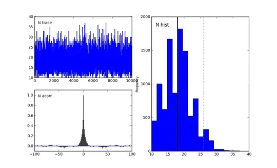
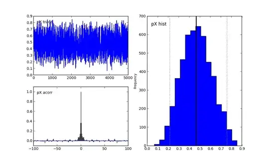
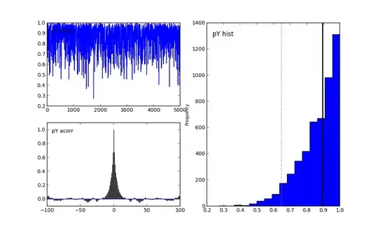
Let's examine the first graph for $N$. The N Trace graph are the samples, in order, I generated from the posterior distribution. The N acorr graph is the auto-correlation between samples. Perhaps there is still too much auto-correlation, and I should burn-in more. Finally, N-hist is the histogram of posterior samples. It looks like the mean is 13. Notice too that no samples were drawn from below 10. This is a good sign, as that would be impossible given the data observed was 5 and 10.

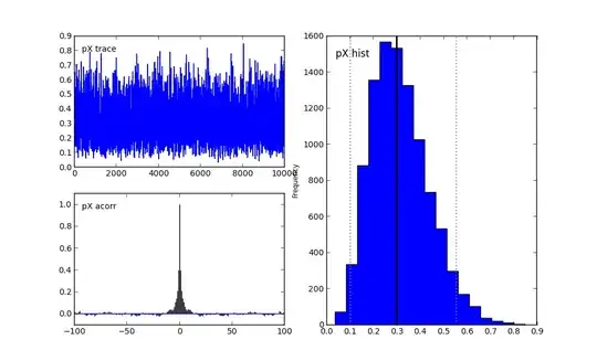
Similar observations can be made for the $pX$ and $pY$ graphs.

enter image description here

enter image description here

enter image description here

Different Prior on $N$

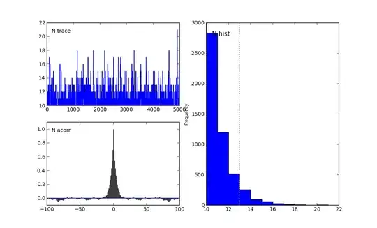
If we restrict $N$ to be a Poisson( 20 ) random variable (and remove the Exponential heirarchy), we get different results. This is an important consideration, and reveals that the prior can make a large difference. See the plots below. Note the time to convergence was much larger here too.

On the other hand, using a Poisson( 10 ) prior produced similar results to the Exp. rate prior.

enter image description here enter image description here enter image description here

Cam.Davidson.Pilon
  • 11,476
  • 5
  • 47
  • 75
  • 1
    I should note that I tried the same analysis with an uninformative prior on $N$ and got terrible results (chain did not converge to anything meaningful, and autocorrelations spiked). – Cam.Davidson.Pilon Jan 07 '13 at 22:11
  • 1
    This looks really good--thanks. I hadn't been able to figure out what to do with _N_, but using a Poisson prior with some realism (i.e., >max(_X_,_Y_)) and fitting it too makes sense... and makes it easy to see how I'll calculate the likelihood. :P I'm going to try coding this up in js tomorrow and will almost certainly accept your answer. Thanks again. – neophyte Jan 07 '13 at 22:15
  • +1 @Cam.Davidson.Pilon. This seems to have worked better than I expected. What happens if you give it a more reasonable prior like Poisson(10) or Poisson(20) that has more probability mass in the feasible region above 10? – David J. Harris Jan 07 '13 at 23:35
  • 1
    With a prior of Poisson(10), the results look the same (and convergence is quick), not so with Poisson(20). See edit above. – Cam.Davidson.Pilon Jan 08 '13 at 13:14
  • This is great, especially the Poisson examples. Thanks so much! – neophyte Jan 08 '13 at 15:04
  • Okay, the posterior is not as obvious as I thought. The point of the conjugate beta priors for px and py is to calculate the posterior directly from the Beta distribution. I don't understand exactly where the priors for N should enter. This might deserve a separate question--actually writing the code is revealing to me the true depths of my ignorance. – neophyte Jan 08 '13 at 22:26
  • Well, we need to include $N$ somehow, as we do not know its value beforehand. The postierior looks like: $P(px,py | X,Y ) \propto P(X | px, N)P(Y | py, N) P(px)P(py)P(N)$. – Cam.Davidson.Pilon Jan 09 '13 at 13:13
  • 1
    Bayesian methods are quite difficult in the details. The overall picture is easy: *Return a distribution of the parameter in question, given the data and prior*, but the small details like: *how to sample*, *what to do with samples*, *what do I need to calculate* and so on can be intimidating. It took me three straight days staring at a computer screen to finally break through ahha – Cam.Davidson.Pilon Jan 09 '13 at 13:16