To take the second question first - what is a 95% credibility interval (no longer a confidence interval, now we are in the Bayesian world) for the probability that a person receiving the treatment will die (this seems to be the "actual value" you are calculating a confidence interval for in your line of code starting > pbar = A/N;).
As you seem to be aware, Laplace favoured using a uniform prior distribution (with p taking a value in [0,1]) for this sort of problem with proportions. A uniform distribution over [0,1] is a beta(1,1) distribution, which has the advantage of being a conjugate prior distribution for p; ie once you modify the distribution based on your observation, the resulting posterior distribution will have the same form as the prior - a beta distribution of some sort. Any textbook will show that this means the posterior distribution for p will be beta (A+1, N-A+1). From here you can just use this distribution as the basis for calculating your credibility interval - there is no need to use monte carlo techniques so long as you have access to tables or software that can calculate the relevant values from the beta distribution.
This will generally give you similar results to your frequentist approach relying on the central limit theorem for the distribution of pbar to approximate normal, as in your code snippet. See for example:
> options(digits=3)
> A <- 100
> N <- 10000
>
> # Frequentist approach, using approximation to Normal:
> pbar = A/N; se = sqrt(pbar * (1-pbar)/N); e = qnorm(.975)*se; pbar + c(-e, e)
[1] 0.00805 0.01195
>
> # Bayesian approach, with uniform prior:
> qbeta(c(0.025, 0.975), A+1, N-A+1)
[1] 0.00823 0.01215
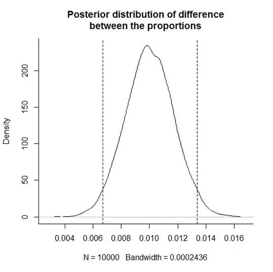
Now, things are a little more complicated if you're really interested in the difference (not in what your one line snipped had) ie you want the posterior distribution and hence a credibility interval for the difference in probability of dying between the treatment and control populations, but the principles are the same. As you suggest and Greg Snow says in his answer, if you can't be bothered calculating the exact posterior distribution of the difference between the propostions why not use simulation? Certainly there's less paperwork involved; and it has the advantage of being easily extendible to more complex comparisons of the estimated posterior distributions of independent parameters:
> A <- 100
> N <- 10000
> B <- 200
> M <- 10000
> sim <- rbeta(10000, B+1, M-B+1) - rbeta(10000, A+1, N-A+1)
> quantile(sim, c(0.025, 0.975))
  2.5%  97.5%
0.0067 0.0134
> plot(density(sim), bty="l", main="Posterior distribution of difference\nbetween the proportions")
> abline(v=quantile(sim, c(0.025, 0.975)), lty=2)
Your first question was about hypothesis testing. Typically choosing between two hypotheses is done by comparing the posterior and prior odds ratios of the two hypothesis ie by calculating the Bayes factor:
$\frac{P(H_0|z)/P(H_1|z)}{P(H_0)/P(H_1)} $
where z is the observed data.
From here it gets a little complicated. Exactly how the two hypotheses are formulated is important - in a case such as yours it will generally be necessary to have $H_1$ indicating the treatment proportion is more than a specified amount different than the original - because under the prior distribution of the continuous random variable p the chance of any exact equivalence of the two is zero (a problem with "sharp" hypotheses). I'd consult a text to see how this plays out, but hopefully this was enough to get you started.