How to Assess Linearity assumption of logit in logistic regression

Question

In Applied Lineare Regression, (Hosmer, Lemeshow, Sturdivant 3rd ed.) Ch. 4, they present "Purposeful Selection." Part of step 5 is to assess the validity of the linearity assumption of the logit vs the covariates. To do this, they fit their model, and then somehow plot the logit as a continuous function against a continuous covariate to see if it fits the linear model

$$g(\pi) = \beta_0 + \beta_1 x_2 + \cdots$$

In OLS, one would simply plot the DV against an IV to see if it is appears linear. In logistic regression the DV is dichotomous, so this doesn't work.

Given data where one of the continuous variables is NOT linear with the logit, how do I create an image such as figure 4.1 (p. 114, 3rd ed.)?

I created a simulation below to demonstrate my issue, and provide a framework of help.

How given that I have fit my simulated data with a simple linear model, how would I take my fitted data and generate a plot that shows the nonlinear nature of the variable Y?

Define parameters

### Size of population
N = 1000

### Create Independent variables
low = 0
high = 5
R = seq(0,5,(high-low)/(N-1))

X = sample(R, N, replace=T)
Y = sample(R, N, replace=T)

### Model parameters
b_0 = -2
b_x = -0.2
b_y = 0.3

Define the model

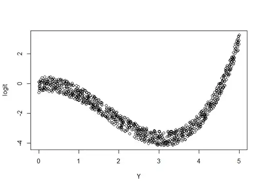
logit  = b_0 + b_x*X + b_y*(Y+1)*(Y-2)*(Y-4)
p = 1/(1 + exp(-logit))
plot(logit~Y)

Sample the data

### Sample the data
Z = rbinom(N, 1, p)
Z = factor(ifelse(Z==0, "No", "Yes"),levels=c("No", "Yes"))

### Create dataframe
df = data.frame(
  X = X,
  Y = Y,
  Z = Z,
  logit = logit,
  p = p
)

Naive Regression

######  Naive Model
### Perform regression
print(sprintf("b_0: %s, b_x: %s, b_y: %s", b_0, b_x, b_y))
#> [1] "b_0: -2, b_x: -0.2, b_y: 0.3"

logfit = glm(Z ~ Y + X, df, family=binomial)
summary(logfit)
#> 
#> Call:
#> glm(formula = Z ~ Y + X, family = binomial, data = df)
#> 
#> Deviance Residuals: 
#>     Min       1Q   Median       3Q      Max  
#> -0.8982  -0.7527  -0.6768  -0.5838   1.9656  
#> 
#> Coefficients:
#>             Estimate Std. Error z value Pr(>|z|)    
#> (Intercept) -1.00404    0.20164  -4.979 6.38e-07 ***
#> Y            0.07223    0.05162   1.399  0.16175    
#> X           -0.15893    0.05288  -3.006  0.00265 ** 
#> ---
#> Signif. codes:  0 '***' 0.001 '**' 0.01 '*' 0.05 '.' 0.1 ' ' 1
#> 
#> (Dispersion parameter for binomial family taken to be 1)
#> 
#>     Null deviance: 1078.6  on 999  degrees of freedom
#> Residual deviance: 1067.4  on 997  degrees of freedom
#> AIC: 1073.4
#> 
#> Number of Fisher Scoring iterations: 4

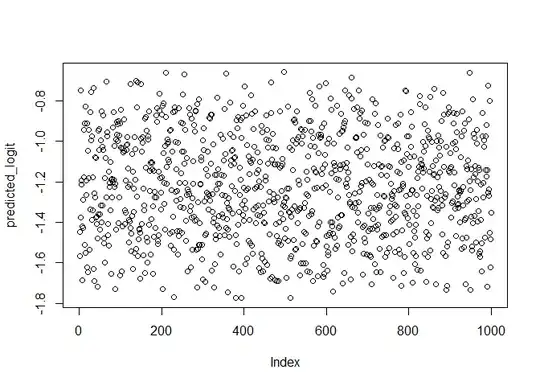
### Plot Y vs predicted logit
predicted_logit = predict(logfit, df)
plot(predicted_logit)

"Correct" Regression

##### "Correct" Model

print(sprintf("b_0: %s, b_x: %s, b_y: %s", b_0, b_x, b_y))
#> [1] "b_0: -2, b_x: -0.2, b_y: 0.3"

logfit = glm(Z ~ X + I((Y+1)*(Y-2)*(Y-4)), df, family=binomial)
summary(logfit)
#> 
#> Call:
#> glm(formula = Z ~ X + I((Y + 1) * (Y - 2) * (Y - 4)), family = binomial, 
#>     data = df)
#> 
#> Deviance Residuals: 
#>     Min       1Q   Median       3Q      Max  
#> -1.9261  -0.6206  -0.3072  -0.1875   2.8250  
#> 
#> Coefficients:
#>                                Estimate Std. Error z value Pr(>|z|)    
#> (Intercept)                    -1.97978    0.20493  -9.661  < 2e-16 ***
#> X                              -0.21401    0.06275  -3.411 0.000648 ***
#> I((Y + 1) * (Y - 2) * (Y - 4))  0.29018    0.02165  13.404  < 2e-16 ***
#> ---
#> Signif. codes:  0 '***' 0.001 '**' 0.01 '*' 0.05 '.' 0.1 ' ' 1
#> 
#> (Dispersion parameter for binomial family taken to be 1)
#> 
#>     Null deviance: 1078.55  on 999  degrees of freedom
#> Residual deviance:  777.76  on 997  degrees of freedom
#> AIC: 783.76
#> 
#> Number of Fisher Scoring iterations: 5

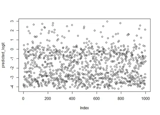
### Plot Y vs predicted logit
predicted_logit = predict(logfit, df)
plot(predicted_logit)

^{Created on 2020-05-27 by the reprex package (v0.3.0)}