1

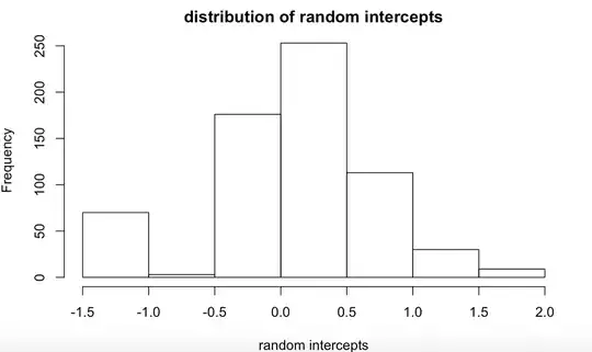
My model gives me random intercepts in which the distribution looks like: enter image description here

The model is as follows: mod <- lmer(response ~ 0 + item + (1|id), family = binomial)

Is this still a valid random effects distribution or does this indicate that there's something wrong with my model ?

Edit: this is the distribution of the random intercept of the model above. It was extracted using ranef() in R. This is what it looks like in the bigger picture.

enter image description here

When I increase the bin size, it looks like this: enter image description here
Edit2: This model is an Item Response (IRT) model (or Rasch) Basically I have a list of patients and their answers to several survey questions. The answers of this survey are binary (e.g. do you exercise at least once a week, etc)

This then transformed into item-response format (wide: patient_id, Q1, Q2, ...Qn to long: patient_id, item (which is Q1,..,Qn) and response (which is the answers to the item column)

Then I fit this data into IRT above, extract the random intercepts as an indices to measure their health level (sort of)
user282983
  • 23
  • 3
  • How does histogram of this data look? Or density plot with bigger bandwidth? – Tim May 22 '20 at 10:10
  • How many observations did you plot? KDEs are useful but can look multimodal when there are not many observations. – Dave May 22 '20 at 10:36
  • @Tim the density above has bandwith = 0.1219, if I increase it to 1 then it'll look fairly normal to me, if 2, then it'll be completely normal (i use plot(density(data)) btw). However, I'm not sure if the determination of whether the random effects look normal is as flexible as that. For histogram, it also looks kinda normal if the bin set to be 0.5. – user282983 May 22 '20 at 12:40
  • @Dave isn't density function in r implement KDE? – user282983 May 22 '20 at 12:40
  • It does! Isn’t that what you did, something like plot(density(observations))? – Dave May 22 '20 at 12:50
  • @Dave yes, but something like plot(density(rep(c(1,2), 50))) will give you a bimodal distribution and as you increase the width, it'll become normal, so basically any data can become normal if you increase the width enough – user282983 May 22 '20 at 12:53
  • Well, this is how kernel density estimator behaves when you change the bandwidth. When you change it to very small values, it has multiple "hills", if it is big, it becomes "smooth". See: https://stats.stackexchange.com/questions/244012/can-you-explain-parzen-window-kernel-density-estimation-in-laymans-terms/244023#244023 – Tim May 22 '20 at 13:17
  • Also, you didn't tell us what exactly does the plot show, so maybe I'm missing something and if the above does not answer your concerns, you need to edit your question and give us more details: (1) how exactly did you produce the plot? (2) label the x-axis, (3) best: show histogram, etc. – Tim May 22 '20 at 13:20
  • I think it's maybe best to show the distinct values that you have, and not even bin them. – Nick Cox May 22 '20 at 14:04
  • Also, tell us more about your data: what it is? What is your model about? – Tim May 22 '20 at 14:15
  • @Tim thank you for the info request. This is the distribution of random intercepts from glmer(response ~ 0 + item + (1|patient_id)); this is GLMM version of Rasch Model or IRT. So each patient will have an index coefficient to measure how healthy they are based on survey questions – user282983 May 22 '20 at 14:32

0 Answers0