I was recently trying to figure out what glmnet's ridge regression is doing (7,000 lines of Fortran are no fun) and am confused by its behavior with an uncentered design matrix $X$.
I am aware that there are already a lot of questions on differences between glmnet and manual implementations:
- Why is glmnet ridge regression giving me a different answer than manual calculation?
- Ridge regression results different in using lm.ridge and glmnet
- What are the differences between Ridge regression using R's glmnet and Python's scikit-learn?
The solution usually is that someone forgot to scale $\lambda$ by a factor of $\frac{1}{N}$ or forgot that $y$ is standardized.
However, I try to understand how glmnet handles design matrices with colMeans(X) != 0.
I wrote a small script to demonstrate the problem, where I compare my manual implementation with the penalized and the glmnet packages:
par(mfrow = c(1,2))
set.seed(1)
# Create some dummy data
y <- rnorm(n = 2000)
y <- scale(y)
# not centered on purpose
X <- matrix(rnorm(n = 10 * 2000, mean = 100), nrow = 2000, ncol = 10)
lambda <- 5
# Ridge regression with glmnet
glmnet_fit <- glmnet::glmnet(X, y, family = "gaussian", lambda = lambda, alpha = 0,
standardize = FALSE, intercept = FALSE)
glmnet_coef <- as.numeric(glmnet_fit$beta)
# Ridge via normal equations
manual_coef <- c(solve(t(X) %*% X + diag(lambda * nrow(X), nrow = ncol(X))) %*% t(X) %*% y)
# Ridge with penalized package
penalized_fit <- penalized::penalized(y, penalized = X, unpenalized = ~ 0,
lambda1 = 0, lambda2 = lambda * nrow(X))
#> 12
penalized_coef <- penalized::coef(penalized_fit)
# Compare the results
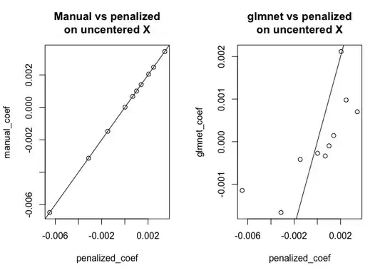
plot(penalized_coef, manual_coef, main = "Manual vs penalized\non uncentered X"); abline(0,1)
plot(penalized_coef, glmnet_coef, main = "glmnet vs penalized\non uncentered X"); abline(0,1)
##### Normalized X
X_norm <- scale(X)
# Ridge regression with glmnet
glmnet_fit <- glmnet::glmnet(X_norm, y, family = "gaussian", lambda = lambda, alpha = 0,
standardize = FALSE, intercept = FALSE)
glmnet_coef <- as.numeric(glmnet_fit$beta)
# Ridge via normal equations
manual_coef <- c(solve(t(X_norm) %*% X_norm + diag(lambda * nrow(X), nrow = ncol(X))) %*% t(X_norm) %*% y)
# Ridge with penalized package
penalized_fit <- penalized::penalized(y, penalized = X_norm, unpenalized = ~ 0,
lambda1 = 0, lambda2 = lambda * nrow(X))
#> 12
penalized_coef <- penalized::coef(penalized_fit)
# Compare the results
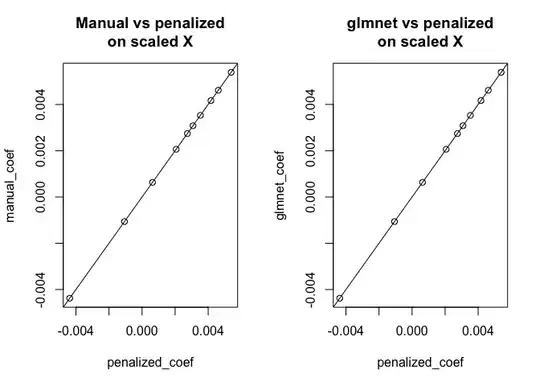
plot(penalized_coef, manual_coef, main = "Manual vs penalized\non scaled X"); abline(0,1)
plot(penalized_coef, glmnet_coef, main = "glmnet vs penalized\non scaled X"); abline(0,1)
Created on 2020-05-16 by the reprex package (v0.3.0)
As you can see, for centered $X$ the results agree between all three approaches, however for uncentered $X$ glmnet is doing something different. (I also did check the behavior with standardize = TRUE, but that doesn't change the problem.)
If anyone has some insight on what I missed or what glmnet is doing internally, I would be very thankful :)