Acceptance- rejection-method with a uniform distribution

Question

In the inversion method, when generating $Y$ from $g(y)$, do you just make $U$ equal to the function $g(y)$, then find the inverse (seen in notes) or are you meant to find the CDF or $g(y)$, then make that equal to $U$, because the $g(y)$ I have is an constant and I can't find a $Y$ from that.

My $f(x)= 1/c(x^2+a)$ and my $g(x)=1/2$, I think its a half anyway, the questions says' construct the acceptance-rejection approach for $f$ using samples from the Uniform distribution in $(−1, 1)$.' And doesn't the inversion method say that $U$ should be distributed on $(0,1)$, what do I do with $U(1,1)$

Answer 1

"when generating $Y$ from $g(y)$"

This sentence does not tell what $g(\cdot)$ stands for: it could be the cdf, the pdf, the mgf, the characteristic function, the quantile function.

"the inversion method"

This simulation method amounts to

1. Generate a uniform $U(0,1)$ variate $U$
2. Compute $Y=Q(U)=F^{-1}(U)$

where $F(\cdot)$ is the cdf of $Y$ and $Q(\cdot)$ is its inverse, namely the quantile function.

construct the acceptance-rejection approach for $f$ using samples from the Uniform distribution in $(−1,1)$

There is a confusion between the inversion method (see above) and the accept-reject method: the latter operates by choosing another distribution with density $f(\cdot)$ to generate from a distribution with density $g(\cdot)$ as follows:

1. Generate $X$ with density $f(\cdot)$
2. Generate an independent uniform $U(0,1)$ variate $U$
3. Set $Y=X$ if $U\le f(X)/g(X)\big/\sup_x \{f(x)/g(x)\}$, else return to 1.

In the current example this means

1. Generate $X$ with Cauchy density $f(x)=\sqrt{a}/\pi (a+x^2)^{-1}$
2. Generate an independent uniform $U(0,1)$ variate $U$
3. Set $Y=X$ if $U\le \mathbb{I}_{(-1,1)}(X)(a+X^2)\big/\sup_{-1\le x\le 1}(a+x^2)$, else return to 1.

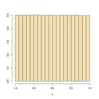
Here is an illustration that the method works, based on 10⁶ replications of

x=rcauchy(1)
while(runif(1)>(x^2<1)*(1+x^2)/2) x=rcauchy(1)

I strongly suggest investing in reading the relevant chapter of a simulation textbook to overcome these confusions.