5

Is there a way to set a boundary constraint when one uses smoothing splines?

For example, I usually fit the data with the following code using the R package mgcv :

library(mgcv)
x <- runif(100, 1, 9)
y <- sin((x^2)/10)+rnorm(100)
plot(gam(y~s(x)))

Suppose I would like to set a boundary constraint at the two points of x at 0 and 10 so that y = 0 when x = 0, 10. Notice that the two end points are outside the range [1, 9] of x. Is this achievable with mgcv?

bluepole
  • 2,376
  • 3
  • 25
  • 34
  • 1
    Did you try the 'pc' argument in s() function? – Gi_F. Apr 24 '20 at 07:59
  • 1
    @Gi_F. This doesn't appear to work for multiple point constraints – Gavin Simpson Apr 24 '20 at 16:59
  • @GavinSimpson @Gi_F. It seems working to some extent. The plotting only shows the fitted curve within the range of `x` values and does not extend to the constraint data points, but the extrapolation looks to meet the constraint. Also, the fitting would be changed to some extent with a much worse uncertainty band (I guess it's expected). – bluepole Apr 24 '20 at 17:31
  • @bluepole Pretty sure it doesn't work for multiple points as per your question. Try: `sim – Gavin Simpson Apr 24 '20 at 19:16

2 Answers2

5

As pointed in the comments, the pc argument of the s() function included in the mgcv package does not allow for multiple constraint points. This is unfortunate but I think should not be too complicated to achieve the objective outside the realm of the specific package.

Intro

I think we can obtain the result we wish using two strategy:

  • approximate the conditions (we will not get exactly $y = 0$ at $x = [0, 10]$)
  • exact constraints

The first strategy has the advantage to allow for easy inference and can also be easily translate in Bayesian settings if one wish so (and might also be possible to achieve within mgcv but I am not a super expert of the package). However I will not go so much into the details but I will point to some reference.

I will discuss both solutions using P-splines smoothing as introduced by Eilers and Marx, 1991 (option bs = ps in s() function). P-splines combine B-spline bases and finite difference penalties (you can read more about this here and here...please give a look at the extrapolation properties of the P-splines because it is relevant in your case).

In what follows I will indicate with $B$ a matrix of B-spline bases, with $P$ a finite difference penalty matrix and with $\lambda$ the smoothing parameter (I will keep it fixed for convenience in the codes).

Strategy 1 - extra penalty

This 'trick' consists in adding an extra penalty term to the penalized problem. The penalized least squares problem becomes then $$ \min_{c} S_{p} = \|y - B c\|^{2} + \lambda c^{\top} P c + \kappa (\Gamma c - v(x_{0}))^{\top} (\Gamma c - v(x_{0})) $$ where $\Gamma$ is the B-spline functions evaluated at the boundary points, $\kappa$ is a large constant (say $10^8$) and $v(x_{0})$ are the boundary abscissa (n your case a vector of zero of dim 2).

Strategy 2 - Lagrange multipliers

The previous strategy gives only a sort of 'soft' approximations. We can obtain an exact match using Lagrange multipliers (a reference in this context is here). In this case the penalized least squares problem is slightly different: $$ \min_{c} S_{l} = \|y - B c\|^{2} + \lambda c^{\top} P c + \gamma^{\top} (\Gamma c - v(x_{0})) $$ where $\gamma$ is a vector of Lagrange multipliers to be estimated.

A small R code

I will now use both strategies to smooth your data. I hope the code is clear enough (anyway I left some comments to guide you). The code supposes that you have a function to compute the B-splines $B$ (see for example Eilers and Marx, 2010).

  rm(list =ls()); graphics.off()

  # Simulate some data
  set.seed(2020)
  xmin = 1
  xmax = 9
  m    = 200
  x    = seq(xmin, xmax, length = m)
  ys   = sin((x^2)/10)
  y    = ys+rnorm(m) * 0.2

  # Boundary conditions
  bx = c(0, 10)
  by = c(0, 0)

  # Compute bases for function, first and second derivative 
  bdeg = 3
  nseg = 50
  B0 = bbase(x, bx[1], bx[2], nseg, bdeg)
  nb = ncol(B0)
  Gi = bbase(bx, bx[1], bx[2], nseg, bdeg)


  # Set syste penalty and  with extra penalty
  D   = diff(diag(nb), diff = 2)
  P   = t(D) %*% D
  Bb  = t(B0) %*% B0
  Ci  = t(Gi) %*% Gi
  lam = 1e1
  kap = 1e8

  # Solve system strategy 1
  cof_p = solve(Bb + lam * P + kap * Ci) %*% (t(B0) %*% y + kap * t(Gi) %*% by)

  # Solve system strategy 2
  LS = rbind((Bb + lam * P), Gi)
  RS = rbind(t(Gi), 0 * diag(0, nrow(Gi)))
  cof_l = solve(cbind(LS, RS)) %*% c(t(B0) %*% y, by)

  # Plot results
  plot(x, y, xlim = bx, pch = 16)
  lines(x, ys, col = 8, lwd = 2)
  points(bx, by, pch = 15)

  # Strategy 1
  lines(x, B0 %*% cof_p, lwd = 2, col = 2)
  points(bx[1], (Gi %*% cof_p)[1], col = 2, pch = 16)
  points(bx[2], (Gi %*% cof_p)[2], col = 2, pch = 16)

  # Strategy 2
  lines(x, B0 %*% cof_l[1:nb], lwd = 2, col = 3, lty = 2)
  points(bx[1], (Gi %*% cof_l[1:nb])[1], col = 3, pch = 16, cex = 0.75)
  points(bx[2], (Gi %*% cof_l[1:nb])[2], col = 3, pch = 16, cex = 0.75)

  legend('bottomleft', c('data', 'signal', 'strategy1', 'strategy2'), col = c(1, 8, 2, 3), pch = 16)

The final results should look like this: enter image description here

I hope this helps somehow.

Gi_F.
  • 1,011
  • 1
  • 7
  • 11
  • 1
    Thanks a lot! This does seem to address the posted question, but I'll have to take some time digesting your code. My ultimate goal is actually to extend it to the situation with random-effects components. Do you think that your solution could be applied to a scenario like gamm4(value ~ s(time, pc=c(0,10)), data=dat, random=~(1|subject))? – bluepole Apr 24 '20 at 19:45
  • Well the first strategy can be useful I think. I know of somebody using it in a Bayesian setting (see https://link.springer.com/article/10.1007/s10182-015-0257-5). The context is totally different but it could give you a hint at least. – Gi_F. Apr 24 '20 at 19:50
  • 1
    @bluepole I was thinking a bit about your last comment and I have a question. If I understood it well you would like to have a model with a common smooth effect of time with boundary constraint and a random subject intercept. Is it correct? If yes, I have good news: this can be achieved with strategy 1 but unfortunately not within mgcv (or at least I do not know how with the package). If you are still interested in the issue I could try an answer. – Gi_F. Apr 27 '20 at 14:42
  • Yes, that's what I'd like to achieve. Looking forward to your solution! – bluepole Apr 28 '20 at 01:17
3

This might be a bit long so I will reply in another answer. Following the comment to my previous answer I will attempt a solution to the following problem: fit an additive model with a shared smooth trend effect subject to boundary constraint and a random Id intercept.

Extra penalty in matrix augmentation form

In the comments above I mentioned that strategy 1 of my previous answer can be used to achieve the constrained fit in a GAMM setting. This becomes clear if we write the extra penalty solution in augmented matrix form (in what follows I will use the same notation as in my previous answer). We can say that: $$ \min_{c} S_{p} = \|W^{1/2} (y_{p} - B_{p}c)\|^{2} + \lambda \|D_{d} c\|^{2} $$ where $c$ is a $(m \times 1)$ vector of unknown spline coefficients, $y_{p}$ is a $((n+ 2) \times 1)$ vector obtained stacking the observed $y$ and boundary values $v(x_{0})$, $B_{p}$ is a $((n+2) \times m)$ B-splines basis matrix obtained placing matrices $B$ and $\Gamma$ on top of each other, $W^{1/2}$ is a $((m + 2) \times (m+2))$ diagonal matrix with first $m$ non-zero elements equal to 1 and last two equal to $\sqrt{\kappa}$ and $D_{d}$ is a $d$ order finite difference matrix operator (the penalty matrix is equal to $P = D_{d}^{\top} D_{d}$).

P-splines as mixed models

P-splines (and all the penalized smoothing techniques included in the s() function of the mgcv package) can be written in a linear 'mixed model form'. For P-splines different re-parameterization are possible (see e.g. par 10 of Eilers et al. (2015)). We can for example define

$$ \begin{array}{ll} X = [1, x_{p}^{1}, ..., x_{p}^{d-1}] \\ Z = B_{p}D_{d}^{\top} (D_{d}D_{d}^{\top})^{-1} \end{array} $$ where $x_{p}$ is the $(m+2)$ vector of time points including the last two boundary ordinates. With this in mind we can then rewrite the normal equations for the min problem above as follows (see also this): $$ \left[ \begin{array}{lll} X^{\top} W X & X^{\top} W Z \\ Z^{\top} W X & Z^{\top} W Z + \lambda I \end{array} \right] \left[ \begin{array}{ll} \beta\\ b \end{array} \right] = \left[ \begin{array}{ll} X^{\top} W y_{p} \\ Z^{\top} W y_{p} \end{array} \right] $$ where $\lambda$ is still the smoothing parameter and it is equal to the ratio of variances $\sigma^{2}/\tau^{2}$ with $b \sim N(0, \tau^{2} I)$ and $\epsilon \sim N(0, \sigma^{2} I)$.

Include random intercept

To solve the original problem, we would like to include also a random intercept. This can be achieved by modifying the form of the Z matrix as follows (see also this link ): $$ Z = \left( \begin{array}{lll} Z_{1} ,& \texttt{1}_{1},& 0,& \dots ,& 0 \\ Z_{2} ,& 0,& \texttt{1}_{2},& \dots ,& 0 \\ \vdots ,& \vdots,& \vdots,& \vdots,& \vdots \\ Z_{J} ,& \dots,& \dots, & \dots,& \texttt{1}_{J} \end{array} \right) $$ where $\texttt{1}_{j}$ is a $((n_{j} + 2) \times 1)$ vector of ones used to model the $j-$th subject-specific intercept. Of course this also 'adds' $J$ elements to the vector of random effects $b$ with $\text{Cov}(b) = \begin{pmatrix} \tau^2 \boldsymbol{I} & 0 \\ 0 & \sigma_{\texttt{1}}^2 \boldsymbol{I} \end{pmatrix}$

Small R-code

I will suppose here that you have a function for the definition of the B-spline matrices and their mixed model representation. I left comments and references in the code. In principle, I think this can be achieved within the mgcv package but unfortunately I do not know the package well enough. Instead, I will use nlme package (on which I thing mgcv is written on at least partially).

#####################
# Utility functions #
#####################
Conf_Bands = function(X, Z, f_hat, s2, s2.alpha, alpha = 0.975)
{
# cit: #http://halweb.uc3m.es/esp/Personal/personas/durban/esp/web/cursos/Maringa/gam-markdown/Gams.html#26_penalized_splines_as_mixed_models  
   C        = cbind(X, Z)
   lambda   = s2/s2.alpha
   D        = diag(c(rep(0, ncol(X)), rep(lambda, ncol(Z))))
   S        = s2 * rowSums(C %*% solve(t(C) %*% C + D) * C)
   CB_lower = f_hat - qnorm(alpha) * sqrt(S)
   CB_upper = f_hat + qnorm(alpha) * sqrt(S)
   CB       = cbind(CB_lower, CB_upper)
   CB
}

basesMM = function(B, D, dd, ns, x)
{
 # NB: needs to be modified if n_{j} is different for some j
 Z0 = B %*% t(D) %*% solve(D %*% t(D))
 X0 = outer(x, 1:(dd-1), '^')
 Z  = do.call('rbind', lapply(1:ns, function(i) Z0))
 X  = do.call('rbind', lapply(1:ns, function(i) X0))

 return(list(X = X, Z = Z))
}

#########################
# Utility functions end #
#########################


# Simulate some data
set.seed(2020)
xmin = 1
xmax = 9
m    = 100
x    = seq(xmin, xmax, length = m)
ys   = sin((x^2)/10)
ns   = 3
y    = ys + rnorm(m) * 0.2
yl   = c(-2 + y, -0 + y, 2 + y)
sb   = factor(rep(1:3, each = m))
dat  = data.frame(y = yl, x = rep(x, ns), sub = sb)
  
# Boundary conditions
bx    = c(0, 10)
by    = c(-0, -0)
xfine = seq(bx[1], bx[2], len = m * 2)

# Create bases
# see https://onlinelibrary.wiley.com/doi/10.1002/wics.125
bdeg  = 3
nseg  = 25
dx    = (bx[2] - bx[1]) /nseg
knots = seq(bx[1] - bdeg * dx, bx[2] + bdeg * dx, by = dx)
B0    = bbase(x, bx[1], bx[2], nseg, bdeg)
nb    = ncol(B0)
Gi    = bbase(bx, bx[1], bx[2], nseg, bdeg)
Bf    = bbase(xfine, bx[1], bx[2], nseg, bdeg)

# Penalty stuffs
dd   = 3
D    = diff(diag(1, nb), diff = dd)
kap  = 1e8

# Augmented matrix
Bp = rbind(B0, Gi) 

# Mixed model representation for lme 
# see https://www.researchgate.net/publication/290086196_Twenty_years_of_P-splines
yp       = do.call('c', lapply(split(dat, dat$sub), function (x) c(x$y, by)))
datMM    = data.frame(y = yp)
mmBases  = basesMM(Bp, D, dd, ns, x = c(x, bx))
datMM$X  = mmBases$X
datMM$Z  = mmBases$Z
datMM$w  = c(rep(1, m), 1/kap, 1/kap)
datMM$Id = factor(rep(1, ns * (m + 2)))
datMM$sb = factor(rep(1:ns, each = m + 2))

# lme fit:
# https://www.researchgate.net/publication/8159699_Simple_fitting_of_subject-specific_curves_for_longitudinal_data
# https://stat.ethz.ch/pipermail/r-help/2006-January/087023.html 
# https://stats.stackexchange.com/questions/30970/understanding-the-linear-mixed-effects-model-equation-and-fitting-a-random-effec
fit   = lme(y ~ X, random = list(Id = pdIdent(~ Z - 1), sb = pdIdent( ~ w - 1)), data = datMM, weights = ~w)

# Variance components
s2        =  fit$sigm ^ 2
s2.alpha  =  s2 * exp(2 * unlist(fit$modelStruct)[1])

# Extract coefficients + get fit + value at boundaries
X0        = datMM$X[1:(m+2), ]
Z0        = datMM$Z[1:(m+2), ]
beta.hat  = fit$coef$fixed
b.hat     = fit$coef$random
f.hat     = cbind(1, X0[1:m, ]) %*% beta.hat + Z0[1:m, ] %*% t(b.hat$Id)
f.hatfine = cbind(1,basesMM(Bf, D, dd, ns = 1, x = xfine)$X) %*% beta.hat + basesMM(Bf, D, dd, ns = 1, x = xfine)$Z %*% t(b.hat$Id)
f.cnt     = cbind(1, X0[-c(1:m), ]) %*% beta.hat + Z0[-c(1:m), ] %*% t(b.hat$Id)
fit_bands = Conf_Bands(cbind(1, X0[1:m, ]) , Z0[1:m, ], f.hat, s2, s2.alpha)
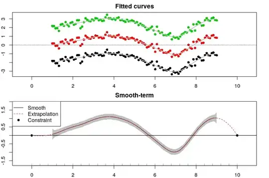
  
# Plots fits
par(mfrow = c(2, 1), mar = rep(2, 4))
plot(rep(x,ns), yl, xlim = range(c(x, bx) + c(-0.5, 0.5)), main = 'Fitted curves', col = as.numeric(dat$sub), pch = 16)
abline(h = 0, lty = 3)
lines(x, f.hat[1:m] + fit$coefficients$random$sb[1], col = 8, lwd = 2)
lines(x, f.hat[1:m] + fit$coefficients$random$sb[2], col = 8, lwd = 2)
lines(x, f.hat[1:m] + fit$coefficients$random$sb[3], col = 8, lwd = 2)

# Plot smooths
plot(x, f.hat, type = 'l', main = 'Smooth-term', xlim = range(c(x, bx) + c(-0.5, 0.5)), ylim = range(fit_bands + c(-0.5, 0.5)))
rug(knots[knots <= bx[2] & knots >= bx[1]])
polygon(x = c(x, rev(x)), y = c(fit_bands[, 1], rev(fit_bands[, 2])), lty = 0, col = scales::alpha('black', alpha = 0.25))
abline(h = by)
points(bx, f.cnt, pch = 16)
lines(xfine, f.hatfine, col = 2, lty = 2)
legend('topleft', legend = c('Smooth', 'Extrapolation', 'Constraint'), col = c(1, 2, 1), lty = c(1, 2, 0), pch = c(-1, -1, 16))

enter image description here

I hope everything here is correct (if you find some mistake, things that are not clear or suggestions please let me know). Finally, I hope my answer will be useful.

Gi_F.
  • 1,011
  • 1
  • 7
  • 11
  • I really appreciate it! This involves a lot of work. Where are the functions `basesMM` and `Conf_Bands` defined? – bluepole Apr 28 '20 at 12:50
  • Sorry forgot to mention: `basesMM` is a wrap for the computation of `X` and `Z` matrices (the formulas are in my answer). The function `Conf_Band` computes the $\alpha \%$ CI for the smooth trend and is equivalent to `Int.Conf` function defined here http://halweb.uc3m.es/esp/Personal/personas/durban/esp/web/cursos/Maringa/gam-markdown/Gams.html#26_penalized_splines_as_mixed_models – Gi_F. Apr 28 '20 at 13:13
  • Thanks a lot for all your help! It will take me a while to digest the whole thing. Do you mind adding the definitions of both `basesMM` and `Conf_Bands` in your code? – bluepole Apr 28 '20 at 13:45
  • 1
    Hi I added the functions you asked for. Anyway notice that the entire procedure does not change much if, for example, you will use TPFs bases (which is `s()` with `bs = 'tp'`). Just hope this helps you. – Gi_F. Apr 28 '20 at 14:02
  • 1
    Anyway, trust me when I say that the R-code is not relevant...I am pretty sure you could get the same results (I hope at least they would be the same) by using `mgcv` in the right way (it is just that I do not know how) – Gi_F. Apr 28 '20 at 14:09
  • Perfect! Thanks again for your kind help. – bluepole Apr 28 '20 at 16:25