Probability of Crossing a Threshold as a Function of Time (Forward Model)

Question

I know the state of some object at a given time. Let's assume that the state is temperature. At each time, I also know the mean and variance of that temperature. I would like to obtain a probability estimate of when the temperature of that object crosses a particular threshold $T_t$.

Here are some simple examples to work with:

Linear: $T(t) = kt \pm ct$ where $k$ is the slope of the line and $c$ is the uncertainty in the measurement, which grows as time moves further from zero.

Nonlinear: $T(t) = kt^2 \pm ct$ where only the main data and not the errors have a nonlinear dependence on time.

Questions: How do I find the probability that the line passed $T_t$ at each time? Or is there a better way to state this?

These two equations are not regressions, but forward models that account for unmodelled effects. That is where the uncertainties come in. If I need to provide more detail on what I mean, please let me know.

NOTE: IF THERE IS NOT ENOUGH INFORMATION HERE, PLEASE ADD A COMMENT STATING WHAT YOU WOULD LIKE CLARIFIED WHEN TEMPORATILY CLOSING THE QUESTION AND PLEASE ONLY DO SO IF YOU ARE WILLING TO RESPOND TO THE COMMENTS I MAKE IN RETURN.

Answer 1

So, after thinking this my own question over, I have come up with the following solution. I first list the steps I took, the output figure, and the python code I used to generate that figure. I look forward to anyone's feedback on whether this is a legitimate method for solving the problem.

Steps:

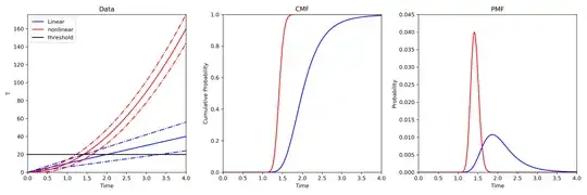
1. Calculate $T(t)$ for linear and nonlinear models.
2. Calculate the probability that the model is above the threshold at every time step. This provides the cumulative mass function for whether the model has crossed the threshold.
3. Calculate the probability mass function from the CMF.

Figure: Code:

import numpy as np
import matplotlib.pyplot as plt
import scipy.stats

# set time domain
t0 = 0
tf = 4
ts = 0.01
tnum = int((tf-t0)/ts+1)
t = np.linspace(t0, tf, tnum, endpoint=True)

# params
k = 10
c = 4
threshold = 20

# linear function
T_linear = np.zeros(tnum)
T_linear_h = np.zeros(tnum)
T_linear_l = np.zeros(tnum)
T_linear = k*t
T_linear_h = k*t+c*t
T_linear_l = k*t-c*t

# nonlinear function
T_nlinear = np.zeros(tnum)
T_nlinear_h = np.zeros(tnum)
T_nlinear_l = np.zeros(tnum)
T_nlinear = k*t**2
T_nlinear_h = k*t**2+c*t
T_nlinear_l = k*t**2-c*t

# compute cdf
cdf_linear = np.zeros(tnum)
cdf_nlinear = np.zeros(tnum)
for i in range(tnum):
    iL_mu = T_linear[i]
    iL_sig = (T_linear_h[i]-T_linear[i])/2
    inL_mu = T_nlinear[i]
    inL_sig = (T_nlinear_h[i]-T_nlinear[i])/2
    cdf_linear[i]=1-scipy.stats.norm(iL_mu, iL_sig).cdf(threshold)
    cdf_nlinear[i]=1-scipy.stats.norm(inL_mu, inL_sig).cdf(threshold)

# compute pmf
pmf_linear = np.zeros(tnum)
pmf_linear[0] = cdf_linear[0]
pmf_nlinear = np.zeros(tnum)
pmf_nlinear[0] = cdf_nlinear[0]
for i in range(1,tnum):
    pmf_linear[i] = cdf_linear[i]-cdf_linear[i-1]
    pmf_nlinear[i] = cdf_nlinear[i]-cdf_nlinear[i-1]

# visualize functions
fig = plt.figure(figsize=[15,5])
ax1 = fig.add_subplot(1,3,1)
ax1.plot(t,T_linear, 'b', label='Linear')
ax1.plot(t,T_linear_h, 'b-.')
ax1.plot(t,T_linear_l, 'b-.')
ax1.plot(t,T_nlinear, 'r', label='nonlinear')
ax1.plot(t,T_nlinear_h, 'r-.')
ax1.plot(t,T_nlinear_l, 'r-.')
ax1.axhline(threshold, color='k', label='threshold')
ax1.set_xlim([t0,tf])
ax1.set_ylim([0, np.max(T_nlinear_h)])
ax1.set_xlabel('Time')
ax1.set_ylabel('T')
ax1.set_title('Data')
ax1.legend()

# visualize cdf
ax2 = fig.add_subplot(1,3,2)
ax2.plot(t,cdf_linear, 'b')
ax2.plot(t,cdf_nlinear, 'r')
ax2.set_xlim([t0,tf])
ax2.set_ylim([0, 1])
ax2.set_xlabel('Time')
ax2.set_ylabel('Cumulative Probability')
ax2.set_title('CMF')

# visualize pmf
ax3 = fig.add_subplot(1,3,3)
ax3.plot(t,pmf_linear, 'b')
ax3.plot(t,pmf_nlinear, 'r')
ax3.set_xlim([0,4])
ax3.set_ylim([0, 0.045])
ax3.set_xlabel('Time')
ax3.set_ylabel('Probability')
ax3.set_title('PMF')

fig.tight_layout()