Multilevel model with perfectly correlated intercept and slope

Question

Setup

Take a simple mixed model with random intercepts and random slopes. I would like to know how the R package nlme can be forced to assume perfectly correlated random intercepts and slopes.

The following code can generate data for the four model types listed below.

library(data.table)
library(MASS)
library(ggplot2)
library(nlme)

make.data <- function(n_id, n_x, var_intercept, var_slope, 
  cor_intercept_slope, noise) {
  id <- seq(n_id)
  x <- seq(0, n_x)
  mu <- c(0, 0)
  cov_intercept_slope <- cor_intercept_slope * sqrt(var_slope 
    * var_intercept)
  sigma <- matrix(c(var_intercept, cov_intercept_slope, 
                   cov_intercept_slope, var_slope), 2, 2)
  data <- CJ(id = id, x = x)
  data[, y_line := apply(mvrnorm(1, mu, sigma) * rbind(rep(1, 
        n_x + 1), x), 2, sum), by = id]
  data[, y_points := y_line + rnorm(.N, 0, noise)]
  return(data)
}

make.plot <- function(data) {
  ggplot(data = data[id <= 7 & x <= 15]) +
    geom_line(mapping = aes(x = x, y = y_line, col = 
        factor(id))) +
    geom_point(mapping = aes(x = x, y = y_points, col = 
          factor(id))) +
    ylim(-4, 4)
}

Random intercept only

In case of a mixed model with only a random intercept, the data may look something like the graph below.

data_intercept <- make.data(10^3, 10^2, 1.9, 0.0, 0.0, 0.1)
make.plot(data_intercept)

To fit this data using nlme, the following formula can be used. There are two unknowns to be estimated; the size of the random noise and the variance of the random intercepts. These agree with the inputted values.

fit_intercept <- lme(y_points ~ 0, data_intercept, 
         list(id = ~ 1))
VarCorr(fit_intercept)["Residual", "StdDev"] # approx 0.1
VarCorr(fit_intercept)["(Intercept)", "Variance"] 
                                         # approx 1.9

Random slope only

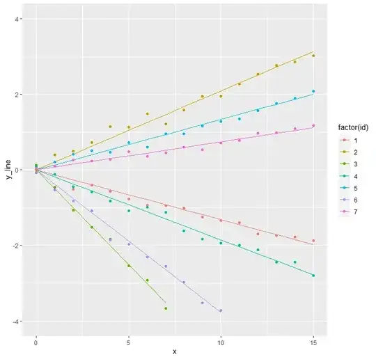
In case of a mixed model with only a random slope, the data may look something like the graph below.

data_slope <- make.data(10^3, 10^2, 0.0, 0.1, 0.0, 0.1)
make.plot(data_slope)

To fit this data using nlme, the following formula can be used. There are two unknowns to be estimated; the size of the random noise and the variance of the random slopes. These agree with the inputted values.

fit_slope <- lme(y_points ~ 0, data_slope, list(id = ~ 0 + 
                  x))
VarCorr(fit_slope)["Residual", "StdDev"] # approx 0.1
VarCorr(fit_slope)["x", "Variance"] # approx 0.1

Random intercept and slope

In case of a mixed model with both a random intercept and a random slope, the data may look something like the graph below.

data_intercept_slope_free <- make.data(10^3, 10^2, 0.8, 0.05, 
                                0.4, 0.1)
make.plot(data_intercept_slope_free)

To fit this data using nlme, the following formula can be used. There are four unknowns to be estimated; the size of the random noise, the variance of the random intercepts, the variance of the random slopes and, finally, the correlation between intercept and slope. These agree with the inputted values.

fit_intercept_slope_free <- lme(y_points ~ 0, 
     data_intercept_slope_free, list(id = ~ 1 + x))
VarCorr(fit_intercept_slope_free)["Residual", "StdDev"] 
            # approx 0.1
VarCorr(fit_intercept_slope_free)["(Intercept)", "Variance"] 
            # approx 0.8
VarCorr(fit_intercept_slope_free)["x", "Variance"] 
            # approx 0.05
VarCorr(fit_intercept_slope_free)["x", "Corr"] # approx 0.4

Random perfectly correlated intercept and slope

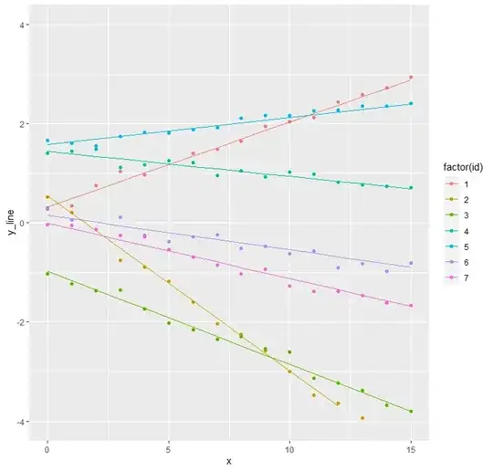
However, one can imagine another model which is nested inside the last model but only has three unknowns to be estimated. If the random intercept and the random slope are perfectly correlated, the data may look something like the graph below.

data_intercept_slope_fixed <- make.data(10^3, 10^2, 0.6, 
   0.05, 1.0, 0.1)
make.plot(data_intercept_slope_fixed)

Theoretically, this is equivalent to the random slopes model, but with the $x$-axis horizontally translated by some value such that the slopes do not cross at $x=0$ but at some other $x=a$. I can imagine this occurring frequently in practice.

Question

• What syntax for the nlme formula can force the correlation to be equal to 1? Something like random = list(id = pdSymm(~ 1 + x, cor = 1)).
• Or alternatively, how can I estimate the horizontal translation in $x$? Something like random = list(id = ~ I(x + a)).

I realise that obtaining a singular fit is generally a sign of overfitting. In my case, I have theoretical grounds to assume this perfect correlation and I am merely interested in obtaining the correct syntax within nlme (if this is even possible).