Let's count the sequences of $n_0$ zeros and $n_1$ ones that begin with a $1$ and have exactly $k$ transitions. Such sequences will contain $k+1$ nonempty groups, of which every odd numbered group consists of ones and the others consist of zeros. Thus, there are $k_1=\lceil (k+1)/2\rceil$ groups of ones and $k_0 = k+1-k_1$ groups of zeros.
A partition of a sequence of length $m$ into $j$ nonempty groups corresponds to a $j-1$ - element subset $\{i_1\lt i_2 \lt \cdots \lt i_{j-1}\}$ of the numbers $\{1,2,\ldots, m-1\}.$ The first group occupies positions $1$ through $i_1;$ the next occupies positions $i_1+1$ through $i_2;$ and so on, until the last group occupies positions $i_{j-1}+1$ through $m.$ Consequently, the number of such partitions is
$$p(m,j) = \binom{m-1}{j-1}.$$
The count of our sequences, then, is the product of the numbers of partitions of the zeros and ones, given by
$$q(k,n_0,n_1) = p(n_1,k_1)\,p(n_0,k_0).$$
The sequences beginning with $0$ are counted by reversing the roles of the zeros and ones. Obviously there is no overlap among these counts. Thus, the total count is
$$f(k,n_0,n_1) = q(k,n_0,n_1) + q(k,n_1,n_0).$$
Because there are $\binom{n_0+n_1}{n_1}$ distinct equally probable permutations (each corresponds to the subset of positions at which ones appear), the probability distribution is given by
$$\Pr(k\text{ transitions}) = \frac{f(k,n_0,n_1)}{\binom{n_0+n_1}{n_1}}.$$
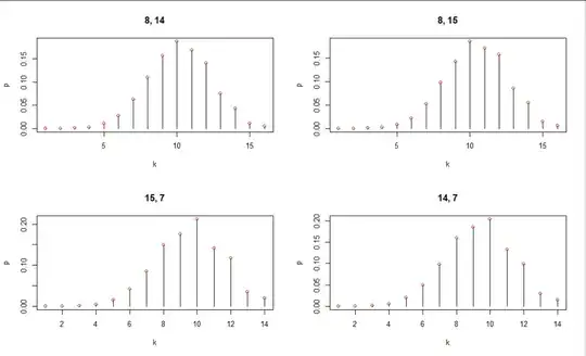
Here are plots of the distribution for selected values of $n_0,n_1$ (as posted in the title of each plot). The red dots are computed using a brute-force enumeration of all the possibilities; they match this calculation exactly.
The binomial coefficients appearing in these formulas can be computed directly rather than recursively. A standard, extremely accurate method uses the formula
$$\binom{n}{k} = \exp\left(\log\Gamma(n+1) - \log\Gamma(k+1) - \log\Gamma(n-k+1)\right)$$
and computes the log Gamma values using Stirling's asymptotic formula (or direct integer arithmetic for small $n$ and $k$).
This is the R code used to implement the formulas and to produce the figure. It computes the logarithms of the two terms in $f$ in order to avoid floating point overflow: later, the log of $\binom{n_0+n_1}{n_1}$ is subtracted from each and the results are exponentiated and added to obtain the probability. This enables computation with fairly high values of $n_0$ and $n_1.$ It takes about three seconds, for instance, to compute 99.99+% of the distribution (the middle $600,000$ values of highest probability) when $n_0=n_1=10^{10}.$
#
# Return the logarithms of the two parts of the function `f`
# (which therefore need to be exponentiated and added to produce a count).
#
f <- function(k, n.0, n.1) {
  lp <- function(m, j) lchoose(m-1, j-1)
  lq <- function(k, n.0, n.1) {
    k.1 <- ceiling((k+1)/2)
    lp(n.1, k.1) + lp(n.0, k + 1 - k.1)
  }
  c(lq(k, n.0, n.1), lq(k, n.1, n.0))
}
#
# Brute force enumeration of permutations of n.0 zeros and n.1 ones,
# returning frequencies of numbers of transitions.
#
f.bf <- function(n.0, n.1) {
  X <- combn(n <- n.0+n.1, n.1)
  zero <- rep(0, n.0+n.1)
  k <- apply(X, 2, function(i) {
    a <- zero
    a[i] <- 1
    sum(a[-n] != a[-1])
  })
  tabulate(k, max(k))
}

par(mfrow=c(2,2))
n <- list(c(8,14), c(8,15), c(15,7), c(14,7))
for (n in n) {
  n.0 <- n[1]
  n.1 <- n[2]
  (p.bf <- f.bf(n.0, n.1))
  k <- seq_along(p.bf)
  #--Compute the probabilities:
  p <- colSums(exp(sapply(k, f, n.0=n.0, n.1=n.1) - lchoose(n.0+n.1, n.0)))
  #--Plot them as bars:
  plot(k, p, type="h", main=paste0(n.0, ", ", n.1))
  points(k, p.bf / choose(n.0+n.1, n.0), col="Red")
}
par(mfrow=c(1,1))
--
