What does dotted line mean in ResNet?

Question

I understand the basic idea of residual neural network (ResNet), just copy $a^{[l]}$ to the add operator at layer $[l+2]$ before the ReLU operator at layer $[l+2]$.

This image shows part of ResNet, which seems to uses 2 types of skip connections, represented by solid line and dotted line respectively.

I would just like to know which one is the copy-paste to $[l+2]$ operation, the solid line or the dotted line.

A post says

The dotted line is there, precisely because there has been a change in the dimension of the input volume (of course a reduction because of the convolution).

What does that mean? Does the dotted line pointed out by red arrow reduce from 64 to 128? I can't understand this. Please help.

Here is the Figure 2. Residual learning: a building block, coming from the ResNet paper.

Answer 1

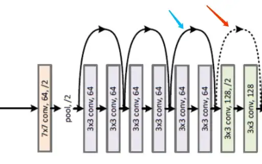
It's best to understand the model in terms of individual "Residual" blocks that stack up and result in the entire architecture. As you would have probably noticed, the dotted connections only come up at a few places where there is an increase in the depth (number of channels and not the spatial dimensions). In this case, the first dotted arrow of the network presents the case where the depth is increased from 64 to 128 channels by 1x1 convolution.

Consider equation (2) of the ResNet paper: $$ y = F(\textbf{x}, \{W_i\}) + W_s \textbf{x} $$ This is used when the dimensions of the mapping function $F$ and the identity function $\textbf{x}$ do not match. The way this is solved is by introducing a linear projection $W_s$. Particularly, as described in page 4 of the Resnet paper, the projection approach means that 1x1 convolutions are performed such that the spatial dimensions remain the size but the number of channels can be increased/decreased (thereby, affecting the depth). See more about 1x1 convolutions and their use here. However, another method of matching the dimensions without having an increase in the number of parameters across the skip connections is to use what is the padding approach. Here, the input is first downsampled by using 1x1 pooling with a stride 2 and then padded with zero channels to increase the depth.

Here is what the paper precisely mentions:

When the dimensions increase (dotted line shortcuts in Fig. 3), we consider two options: (A) The shortcut still performs identity mapping, with extra zero entries padded for increasing dimensions. This option introduces no extra parameter; (B) The projection shortcut in Eqn.(2) is used to match dimensions (done by 1×1 convolutions).

Here are some more references, in case needed - a Reddit thread, another SE question on similar lines.

Answer 2

For a better understanding of the architecture, I'd suggest taking a look at an implementation. There are two types of blocks in the ResNet architecture, keras refers to them as the conv_block and the identity_block.

• The identity_block is the one with the straight line. It consists of three convolution layers (with Batch Norm and a ReLU). The input of the block is added to the last one right before the final activation function. The connection from the input to the add operation is called a skip connection (or a shortcut as keras calls it).
• The conv_block is the one with the dotted line. It two consists the three convolution layers (+BN+ReLU); these are different than the previous, though. The difference is that this time the skip connection passes through an independent convolution layer before being added to the output of the third convolution layer. This layer has a kernel of $1 \times 1$ and uses strides of $2$, which has the effect that changing the dimension of its input.

If you read further down the post you linked to the question, the author does an amazing job of explaining these differences, while giving details about the shapes and dimensions of each layer. I'd definitely recommend reading it, as it will help you clear up the confusion.

Visually to illustrate the difference between the two types of blocks they use the two types of lines: the straight and the dotted one. The straight line is a connection from the input to the output, while the dotted line passes through a convolution layer (which changes its dimensions).