This answer addresses two issues:
No, the distribution of $F_i+\phi_i$ is not Normal. It can be computed exactly because it has a relatively simple formula.
Although the distribution of $Z$ is not Normal, for $N\ge 10$ $Z$ is close to Normally distributed.
The purpose of posting a detailed answer to the second question is to illustrate a careful application of the Central Limit Theorem (CLT). All too often, people assume the CLT's conclusion applies to finite sums (or averages) of independent random variables. This always needs to be verified, because the CLT is only about a limit and says nothing about finite sums.
Here, I conduct the verification through a combination of intuitive heuristics (such as comparing variables to Bernoulli variables), rigorous calculations (to work out the parameters of the approximating Normal distributions), and simulations (to illustrate the results, to provide details that are difficult to compute, and as a check on the calculations).
1. The distribution of $F_i+\phi_i$
Using any of the techniques at Consider the sum of $n$ uniform distributions on $[0,1]$, or $Z_n$. Why does the cusp in the PDF of $Z_n$ disappear for $n \geq 3$?, we may determine that the PDF of each $F_i+\phi_i$ has a trapezoidal shape: it rises linearly from $-50-\pi/4$ to $-50+\pi/4,$ is then horizontal through $0,$ and is symmetric about $0.$ Set $L=50$ and let $g_L$ be this pdf, so that in terms of the CDF $F_L$ of the uniform distribution on $[-L,L],$
$$g_L(x) = F_L\left(x+\frac{\pi}{4}\right) - F_L\left(x-\frac{\pi}{4}\right) = \left\{\begin{array}{ll}
\frac{1}{2L} & |x|\le L-\pi/4 \\ \frac{1}{\pi L}\left(L+\pi/4-|x|\right) & L-\pi/4 \lt x \lt L+\pi/4 \\ 0 & |x| \ge L+\pi/4.
\end{array}\right.$$
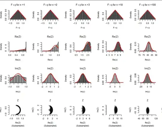
The red curves in the first row of the figure are graphs of $g_{50}.$
2. The (approximate) distribution of $Z$
Because the collection of $F_i+\phi_i$ is independent, their exponentials are independent, too. Splitting them into their real and imaginary parts shows
$$\Re(Z) = \sum_{j=1}^N \cos(F_j+\phi_j);\quad \Im(Z) = \sum_{j=1}^N \sin(F_j+\phi_j).$$
Because sines and cosines are bounded they have finite variances, whence the Central Limit Theorem (CLT) applies. The principal questions are (1) does it really give us an adequate approximation when $N$ is only $10$ and (2) if so, what are the means and variances of the components of $Z$?
Let's generalize a bit and write $50 = L,$ supposing $L\ge \pi/4$ (to avoid examining a separate special case). Because the distribution of $F_i+\phi_i$ is symmetric about $0$ and $\sin$ is an odd function, $\Im(Z)$ must have a symmetric distribution and its mean is zero. Since $2L=100$ is very nearly a whole multiple of $2\pi,$ $\Re(Z)$ must have a nearly symmetric distribution, too, with a mean close to zero. Our familiarity with Bernoulli variables indicates that in such cases the CLT is a decent approximation even with $N$ as small as $5.$ Finally, because $x\to \cos(x)\sin(x)$ is an odd function, the covariance of $\Re(Z)$ and $\Im(Z)$ must be zero: the components of $Z$ are uncorrelated.
The preceding figure illustrates these deductions. It reports on five independent simulations involving ten million values of $F_i+\phi_i$ for each. In each column it displays simulated and theoretical results for various values of $N$ ranging from $1$ to $100.$ The top row is a histogram of the simulated values of $F_i+\phi_i;$ the next two rows are histograms of their cosine and sine (respectively); and the bottom row plots $Z$ itself in the Complex plane (using a 1:1 aspect ratio). The red curves in the top row plot the PDF of $Z_i+\phi_i.$ All the other red curves plot Normal distributions whose parameters are given by the CLT (as I explain below).
Evidently, with $N=10$ the distribution of $Z$ is close to bivariate Normal.
Let's work out the parameters of the Normal approximating distribution. The mean of $\Re(Z),$ for instance, is obtained as
$$\begin{aligned}
E[\Re(Z)] &= N E[\cos(F_i+\phi_i)] = N\int_\mathbb{R} \cos(x)g(x)\,\mathrm{d}x \\
&= N\int_\mathbb{R} \cos(x)\left(F_L(x+\pi/4)-F_L(x-\pi/4)\right)\,\mathrm{d}x \\
&= \frac{N}{2L}\left(\frac{2(4-\pi)\sin(L) + \pi\cos(L)}{\pi\sqrt{2}} + 2\sin(L-\pi/4)\right)
\end{aligned}$$
and its (raw) second moment is
$$E[(\Re(Z))^2] = \frac{N^2}{2L}\left(\frac{4\sin(2L) + 2\pi\cos(2L)+\pi^2)}{4\pi} + L - \frac{\cos(2L) }{2}- \frac{\pi}{4}\right).$$
Subtracting the square of $E[\Re(Z)]$ from this gives the variance. Finally, since the mean of $\Im(Z)$ is zero, its variance equals the raw second moment; and because $\sin^2(x)+\cos^2(x)=1$,
$$\operatorname{Var}(\Im(Z))=\sum_{i=1}^N E[\sin^2(F_i+\phi_i)] = N - \sum_{i=1}^N E[\cos^2(F_i+\phi_i)] = N - E[(\Re(Z))^2] .$$
Notice that these two variances will be equal if and only if the expectation of $\cos(F_i+\phi_i)$ is zero (which happens only when $2L$ is a multiple of $\pi$).
The CLT says that for sufficiently large $N,$ $\Re(Z)$ will approximately have a Normal distribution with mean $E[\Re(Z)]$ and variance $\operatorname{Var}(\Re(Z));$ and $\Im(Z)$ will approximately have a Normal distribution with zero mean and variance $\operatorname{Var}(\Im(Z)).$ Moreover, the covariance of the two components will be zero. These parameters were used to plot the red Normal approximations in the second and third rows of both figures (previously and next).
To appreciate these results, let's examine the extreme case where $L=\pi/4.$
In this case the distribution of $\Re(Z)$ is as skewed as possible, as the plots on the second row indicate. However, even for $N$ as small as $10,$ a Normal approximation looks pretty good. But notice the effect of the nonzero mean, equal to $0.8105695:$ this Normal distribution is shifted far from zero. As a result, the values of $Z$ (bottom row) trace an ellipse-like region centered near $(8,0).$ This ellipse has high eccentricity, because the variances (equal to $29.73$ and $4.56$) have a ratio of $6.52.$
This R code implements the calculations and simulations described here.
n <- c(1, 2, 3, 10, 100)   # Sample sizes to simulate
N <- 1e6           # Minimum number of values per simulation
# L <- pi/4    # Most extreme example
L <- 50        # As in the question
#
# The PDF of F+phi
#
g <- function(x) 2/pi * (punif(x+pi/4, -L, L) - punif(x-pi/4, -L, L))

# (Perform a simple check: is `g` normalized?)
p <- integrate(g, -L-pi/4, L+pi/4, rel.tol=1e-12)$value # Check == 1
(1 - p) # Essentially zero
#
# Moments of exp(1i * (F+phi)).
# (Because sin is an odd function, the mean of the imaginary component is zero.)
# (Because sin(x)*cos(x) is an odd function, the components are uncorrelated.)
# (Commented-out sections verify correctness and consistency of the formulas.)
#
# mu. <- integrate(function(x) cos(x) * g(x), -L-pi/4, L+pi/4, rel.tol=1e-12)
mu <- (2 * (-(pi-4) * sin(L) +   pi * cos(L)) / (sqrt(2) * pi) +
         2 * sin(L - pi/4)) / (2 * L)

# mu2. <- integrate(function(x) cos(x)^2 * g(x), -L-pi/4, L+pi/4, rel.tol=1e-12)
mu2 <- ((4 * sin(2*L) + 2*pi*cos(2*L) + pi^2) / (4*pi) + L -
  cos(2*L)/2 - pi/4) / (2 * L)

v <- mu2 - mu^2 # Variance of the real part
# nu2. <- integrate(function(x) sin(x)^2 * g(x), -L-pi/4, L+pi/4, rel.tol=1e-12)
# nu2 <- ((-4 * sin(2*L) - 2*pi*cos(2*L) + pi^2) / (4*pi) + L +
#           cos(2*L)/2 - pi/4) / (2 * L)
nu2 <- 1 - mu2
w <- nu2        # Variance of the imaginary part
#
# Run the simulations.
#
set.seed(17)
par(mfcol=c(4, length(n)))
for (n in n) {
  n.sim <- ceiling(N / n)
  theta <-  matrix(runif(n * n.sim, -L, L), n) +
    matrix(runif(n * n.sim, -pi/4, pi/4), n)
  z <- colSums(exp(1i * theta))
  #
  # Plot histograms.
  #
  h.x <- hist(Re(z), breaks=50, plot=FALSE)
  h.y <- hist(Im(z), breaks=50, plot=FALSE)

  hist(theta, freq=FALSE, breaks=100,
       main=bquote(paste(F+phi, " for n =", .(n))), xlab=expression(F+phi))
  curve(g(x), add=TRUE, col="Red", lwd=2, n=801)

  ymax <- max(max(h.x$density), dnorm(0,0,sqrt(n * v)))
  plot(h.x, freq=FALSE, ylim=c(0, ymax), main=expression(Re(Z)))
  curve(dnorm(x, mu*n, sqrt(n * v)), add=TRUE, col="Red", lwd=2, n=801)

  ymax <- max(max(h.y$density), dnorm(0,0,sqrt(n * w)))
  plot(h.y, freq=FALSE, ylim=c(0, ymax), main=expression(Im(Z)))
  curve(dnorm(x, 0, sqrt(n * w)), add=TRUE, col="Red", lwd=2, n=801)
  #
  # The scatterplot of the components of `Z`.
  #
  q <- z[seq_len(min(10000, length(z)))] # (R chokes on large datasets)
  plot(Re(q), Im(q), asp=1, bty="n", col="#00000008", main=expression(Z),
       xlab=expression(Re(Z)), ylab=expression(Im(Z)),
       sub="(Subsampled)")
}
par(mfrow=c(1,1))

