I have a dataset where empirical intuition say I should expect a weekly seasonality (i.e., the behavior in saturday and sunday is different from the rest of the week). Should this premise be true, shouldn't an autocorrelation graph give me bursts at lag multiples of 7?
Here's a sample of the data:
data = TemporalData[{{{2012, 09, 28}, 19160768}, {{2012, 09, 19},
    19607936}, {{2012, 09, 08}, 7867456}, {{2012, 09, 15},
    11245024}, {{2012, 09, 04}, 0}, {{2012, 09, 21},
    24314496}, {{2012, 09, 12}, 11233632}, {{2012, 09, 03},
    9886496}, {{2012, 09, 09}, 9122272}, {{2012, 09, 24},
    23103456}, {{2012, 09, 20}, 25721472}, {{2012, 09, 11},
    12272160}, {{2012, 09, 25}, 21876960}, {{2012, 09, 05},
    7182528}, {{2012, 09, 16}, 11754752}, {{2012, 09, 23},
    23737248}, {{2012, 09, 26}, 20985984}, {{2012, 09, 10},
    12123584}, {{2012, 09, 06}, 9076736}, {{2012, 09, 17},
    20123328}, {{2012, 09, 18}, 20634720}, {{2012, 09, 22},
    23361024}, {{2012, 09, 14}, 11804928}, {{2012, 09, 07},
    9007200}, {{2012, 09, 02}, 9244192}, {{2012, 09, 13},
    11335328}, {{2012, 09, 27}, 20694720}, {{2012, 10, 26},
    12242112}, {{2012, 10, 15}, 10963776}, {{2012, 11, 09},
    9735424}, {{2012, 10, 08}, 10078240}, {{2012, 10, 31},
    10676736}, {{2012, 10, 20}, 11719840}, {{2012, 11, 05},
    10475168}, {{2012, 10, 01}, 9988416}, {{2012, 10, 24},
    11998688}, {{2012, 10, 12}, 10393120}, {{2012, 10, 23},
    11987936}, {{2012, 10, 19}, 11165536}, {{2012, 10, 04},
    9902720}, {{2012, 11, 16}, 10023648}, {{2012, 11, 21},
    10047936}, {{2012, 10, 10}, 10205568}, {{2012, 11, 08},
    9872832}, {{2012, 10, 21}, 12854112}, {{2012, 11, 04},
    10485856}, {{2012, 10, 07}, 9565248}, {{2012, 09, 30},
    9784864}, {{2012, 10, 29}, 12880064}, {{2012, 11, 10},
    8945824}, {{2012, 11, 15}, 9870880}, {{2012, 09, 29},
    9718080}, {{2012, 10, 18}, 10992896}, {{2012, 10, 06},
    9319584}, {{2012, 11, 03}, 9077024}, {{2012, 10, 03},
    10537408}, {{2012, 11, 22}, 9853216}, {{2012, 10, 11},
    10191936}, {{2012, 10, 22}, 12766816}, {{2012, 11, 07},
    9510624}, {{2012, 11, 14}, 9707264}, {{2012, 10, 28},
    12060736}, {{2012, 11, 19}, 10946880}, {{2012, 11, 11},
    9529568}, {{2012, 10, 09}, 9967680}, {{2012, 10, 17},
    12093344}, {{2012, 11, 20}, 10520800}, {{2012, 10, 05},
    9619136}, {{2012, 10, 25}, 11484288}, {{2012, 11, 17},
    9389312}, {{2012, 10, 30}, 12078944}, {{2012, 10, 14},
    9505984}, {{2012, 10, 02}, 9943648}, {{2012, 11, 24},
    9458144}, {{2012, 11, 02}, 10082944}, {{2012, 11, 01},
    11082912}, {{2012, 10, 13}, 9117632}, {{2012, 11, 23},
    10253280}, {{2012, 11, 12}, 10240672}, {{2012, 11, 06},
    9723456}, {{2012, 11, 13}, 9806880}, {{2012, 10, 16},
    12368896}, {{2012, 11, 18}, 9632800}, {{2012, 10, 27}, 10606656}}]
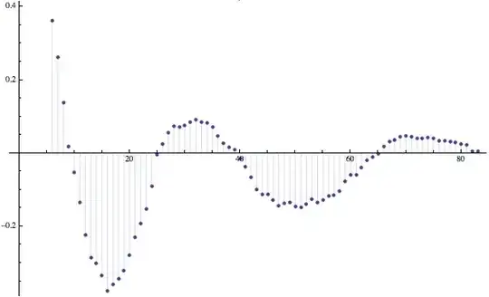
... and the ACF:
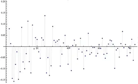
... and the PACF:
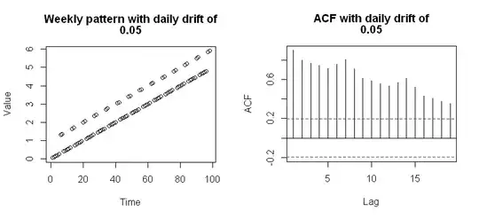
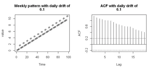
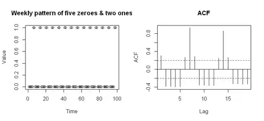 However, this expected ACF pattern can be masked when the data have some trend: